Linear Regression

Notes
- Accuracy
- Outliers & High Leverage points
Exercises

Notes

Accuracy

Residual sum of squares (RSS) = $\sum_{i=1}^n (y_i - \hat{y}_i)^2$.
Residual standard error (RSE) = $\sqrt{\frac{1}{n-2}\text{RSS}}$.
$R^2$ = 1 - $\frac{\text{RSS}}{\text{TSS}}$.
Total sum of squares (TSS) = $\sum_{i=1}^n (y_i - \bar{y}_i)^2$.

Outliers & High Leverage points

Outlier is an observation for which the predicted response is far from the recorded response.
High leverage point is an observation for which the recorded predictors are unusual.
High leverage points usually have more influence on the model than outliers.
The studentized (standardized) residuals are typically expected to be between -3 and 3. If they lie outside then that indicates that there might be outliers in the data.
The average leverage is $(p + 1) / n$. If the leverage of some observation is significantly higher than the average leverage then that is a high leverage point. (Look in to "Cook's distance".)

Exercises

Question 1

Since there are three p-values in Table 3.4, there are three null hypotheses:

H₀⁽¹⁾: sales does not depend on TV
H₀⁽²⁾: sales does not depend on radio
H₀⁽³⁾: sales does not depend on newspaper

The p-values corresponding to the first two null hypotheses are very small, less than 10^-4, whereas the p-value for the last one is close to 1. This means that the probability of seeing the observed sales numbers if H₀⁽¹⁾ or H₀⁽²⁾ is true is almost zero, but the probability of seeing the observed sales numbers if H₀⁽³⁾ is true is almost 1. In other words sales depends on TV and radio but not on newspaper.

Question 2

A KNN classifier classifies an observation is to the class with the majority of nearest neighbors. In the KNN regression method the response is estimated as the average of all the training responses of the nearest neighbors.

Question 3

Assuming X₄ = X₁ X₂ and X₅ = X₁ X₃, the linear fit model is as follows: Y = 50 + 20 X₁ + 0.07 X₂ + 35 X₃ + 0.01 X₁ X₂ - 10 X₃ X₅. Since X₃ (Gender) is 1 for females and 0 for males, this fit essentially gives two models based on the gender: Y = 85 + 10 X₁ + 0.07 X₂ + 0.01 X₁ X₂ for females, and Y = 50 + 20 X₁ + 0.07 X₂ + 0.01 X₁ X₂ for males. If X₁ (GPA), and X₂ (IQ), are fixed for the two genders then the starting salary for males will be more on average than the starting salary of females if X₁ > 35 / 10 = 3.5; i.e. given the GPA is high enough, on average males will have a higher starting salary than females (iii).
If IQ is 110 and GPA is 4.0 then a female is predicted to have a starting salary of $ 137,100.
False. The scale for IQ is much larger than that of GPA or Gender. Hence the coefficients related to any IQ based predictor are expected to be small. (Possibly this is why it is often recommended to scale the predictors, so they are all on an equal footing and it is easier to figure out which ones are important.)

Question 4

Even though the true relationship is linear, we need to take into account the irreducible error $ϵ$. The cubic model is more flexible than the linear model and therefore will be able to better fit to the irreducible error. I expect the cubic model to have lower training RSS than the linear model.
The linear model will have a lower test RSS than the cubic model since it matches the true relationship. The cubic model would have overfitted to the irreducible error in the training data and therefore perform worse on the test data.
Irrespective of the true relationship I would expect the cubic model to have lower training RSS than the linear model because it is more flexible than the linear model and thus fits the training data better.
Since we do not the true relationship between X and Y, it is difficult to say which of the two models will have lower test RSS without more information.

Question 5

We just have to substitute equation 3.38 in to the equation for the $i$th fitted value and rearrange the equation:

\begin{align} a_{i'} = \frac{x_i x_{i'}}{\sum_{k=1}^n x_k^2}. \end{align}

Question 6

The equation for the least squares line is $y = \hat{\beta}_0 + \hat{\beta}_1 x$. From equation 3.4 we have $\hat{\beta}_0 = \bar{y} - \hat{\beta}_1 \bar{x}$. Then putting $x = \bar{x}$ in the least squares line equation we see that $y = \bar{y}$. Thus the least squares line always passes through $(\bar{x}, \bar{y})$.

Question 7

Assumption: $\bar{x} = \bar{y} = 0$. From equation 3.4 we have $\hat{y}_i = \hat{\beta}_1 x_i$, where

\begin{align} \hat{\beta}_1 = \frac{\sum_{i=1}^n x_i y_i}{\sum_{i=1}^n x_i^2}. \end{align}

And from equation 3.17 we have

\begin{align} R^2 = 1 - \frac{\sum_{i=1}^n (y_i - \hat{y}_i)^2}{\sum_{i=1}^n y_i^2}. \end{align}

Expanding the square in the numerator of the above fraction and substituting $\hat{y}_i$ with $\hat{\beta}_1 x_i$ we get

\begin{align} R^2 = \frac{\hat{\beta}_1(2 \sum_{i=1}^n x_iy_i - \hat{\beta}_1 \sum_{i=1}^n x_i^2)}{\sum_{i=1}^n y_i^2}. \end{align}

Now if we simply substitute the above form of $\hat{\beta}_1$ in to this equation we will see that $R^2 = \mathrm{Cor}(X, Y)^2$, where $\mathrm{Cor}(X, Y)$ is given by equation 3.18.

Question 8

Simple linear regression on `Auto` data set

import pandas as pd
import numpy as np
from tabulate import tabulate

auto = pd.read_csv("data/Auto.csv")
print(tabulate(auto.head(), auto.columns, tablefmt="orgtbl"))

|    |   mpg |   cylinders |   displacement |   horsepower |   weight |   acceleration |   year |   origin | name                      |
|----+-------+-------------+----------------+--------------+----------+----------------+--------+----------+---------------------------|
|  0 |    18 |           8 |            307 |          130 |     3504 |           12   |     70 |        1 | chevrolet chevelle malibu |
|  1 |    15 |           8 |            350 |          165 |     3693 |           11.5 |     70 |        1 | buick skylark 320         |
|  2 |    18 |           8 |            318 |          150 |     3436 |           11   |     70 |        1 | plymouth satellite        |
|  3 |    16 |           8 |            304 |          150 |     3433 |           12   |     70 |        1 | amc rebel sst             |
|  4 |    17 |           8 |            302 |          140 |     3449 |           10.5 |     70 |        1 | ford torino               |

Recall from the last chapter horsepower has some missing values and needs to be converted to a numeric form before we can use this for linear regression.

auto.drop(auto[auto.horsepower == "?"].index, inplace=True)
auto["horsepower"] = pd.to_numeric(auto["horsepower"])

For simple linear regression we can use the ordinary least squares model from statsmodels or the linear regression model from scikit-learn. In this question we are asked to print the summary of the fitted model. scikit-learn has no method for generating a summary, but statsmodels does.

import statsmodels.formula.api as smf

model = smf.ols(formula="mpg~horsepower", data=auto).fit()
print(model.summary())

                            OLS Regression Results
==============================================================================
Dep. Variable:                    mpg   R-squared:                       0.606
Model:                            OLS   Adj. R-squared:                  0.605
Method:                 Least Squares   F-statistic:                     599.7
Date:                Mon, 25 May 2020   Prob (F-statistic):           7.03e-81
Time:                        17:19:34   Log-Likelihood:                -1178.7
No. Observations:                 392   AIC:                             2361.
Df Residuals:                     390   BIC:                             2369.
Df Model:                           1
Covariance Type:            nonrobust
==============================================================================
                 coef    std err          t      P>|t|      [0.025      0.975]
------------------------------------------------------------------------------
Intercept     39.9359      0.717     55.660      0.000      38.525      41.347
horsepower    -0.1578      0.006    -24.489      0.000      -0.171      -0.145
==============================================================================
Omnibus:                       16.432   Durbin-Watson:                   0.920
Prob(Omnibus):                  0.000   Jarque-Bera (JB):               17.305
Skew:                           0.492   Prob(JB):                     0.000175
Kurtosis:                       3.299   Cond. No.                         322.
==============================================================================

Warnings:
[1] Standard Errors assume that the covariance matrix of the errors is correctly specified.

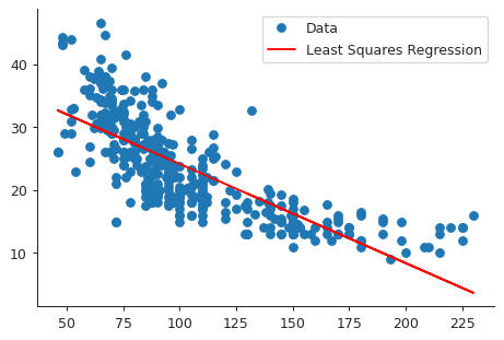
The F-statistic is much larger than 1, and the p-value (P>|t| in the table) is zero. This indicates that there is a relationship between mpg and horsepower.
The $R^2$ value of 0.606 indicates that this relationship explains around 61% of the mpg values.
The coefficient value corresponding to horsepower is negative. This indicates that the relation between mpg and horsepower is negative.

pred = model.get_prediction(exog=dict(horsepower=98))
pred_summary = pred.summary_frame()
print(tabulate(pred_summary, pred_summary.columns, tablefmt="orgtbl"))

|    |    mean |   mean_se |   mean_ci_lower |   mean_ci_upper |   obs_ci_lower |   obs_ci_upper |
|----+---------+-----------+-----------------+-----------------+----------------+----------------|
|  0 | 24.4671 |  0.251262 |         23.9731 |         24.9611 |        14.8094 |        34.1248 |

The predicted mpg for horsepower = 98 is 24.4671. The 95% confidence interval is $[23.9731, 24.9611]$, and the 95% prediction interval is $[14.8094, 34.1248]$. As mentioned in the text, the prediction interval contains the confidence interval.

Least squares plot

import matplotlib.pyplot as plt
import seaborn as sns

sns.set_style("ticks")

X = auto["horsepower"]
Y = auto["mpg"]
Ypred = model.predict(X)

plt.close("all")
fig, ax = plt.subplots()
ax.plot(X, Y, 'o', label="Data")
ax.plot(X, Ypred, 'r', label="Least Squares Regression")
ax.legend(loc="best")
sns.despine()
fig.savefig("img/3_auto_ls.png", dpi=90)

Diagnostic plots

The R command plot in this case gives four diagnostic plots:

Residuals vs Fitted
Normal Q-Q
Scale-Location
Residuals vs Leverage

The Residuals vs Fitted plot shows any non-linear pattern in the residuals, and by extension in the data. The Normal Q-Q plot shows if the residuals are normally distributed. The Scale-Location plot shows if there is heteroscedasticity. The Residuals vs Leverage plot shows if there are leverages in the data.

We will produce these plots using statsmodels and seaborn.

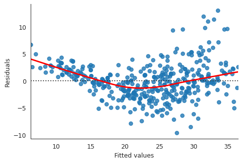
Residuals vs Fitted plot

fitted_vals = model.fittedvalues

plt.close("all")
fig, ax = plt.subplots()
residplot = sns.residplot(x=fitted_vals, y="mpg", data=auto,
                          lowess=True,
                          line_kws={"color": "red"},
                          ax=ax)
ax.set_xlabel("Fitted values")
ax.set_ylabel("Residuals")
sns.despine()
fig.savefig("img/3_res_vs_fit.png", dpi=90)

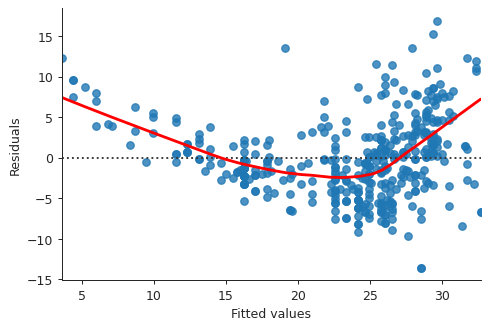
This plot clearly shows that there is non-linearity in the data.

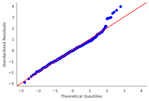
Normal Q-Q plot

import statsmodels.api as sm

residuals = model.resid

plt.close("all")
fig, ax = plt.subplots()
qqplot = sm.qqplot(residuals, line='45', ax=ax, fit=True)
ax.set_ylabel("Standardized Residuals")
sns.despine()
fig.savefig("img/3_auto_qq.png", dpi=90)

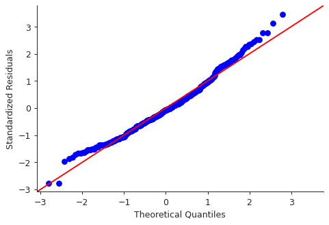
Though there are some points that are far from the $45^\circ$ fitted line, most of the points lie close to the line, indicating that the residuals are mostly normally distributed.

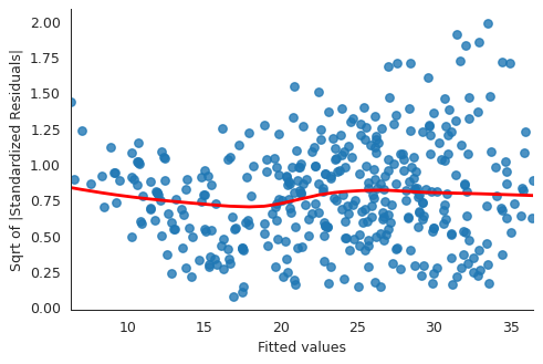
Scale-Location plot

# normalized residuals and their square roots
norm_residuals = model.get_influence().resid_studentized_internal
norm_residuals_abs_sqrt = np.sqrt(np.abs(norm_residuals))

plt.close("all")
fig, ax = plt.subplots()
slplot = sns.regplot(fitted_vals, norm_residuals_abs_sqrt,
                     lowess=True,
                     line_kws={"color" : "red"},
                     ax=ax)
ax.set_xlabel("Fitted values")
ax.set_ylabel("Sqrt of |Standardized Residuals|")
sns.despine()
fig.savefig("img/3_auto_scale_loc.png", dpi=90)

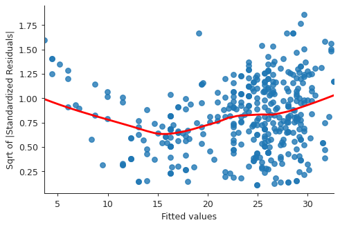
This plot is similar to the first diagnostic plots, except now the quantity on the y-axis is positive. This shows that homoscedasticity is not held, i.e. the variance is not constant.

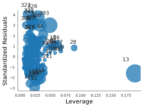
Residuals vs Leverage plot

plt.close("all")
fig, ax = plt.subplots()
rlplot = sm.graphics.influence_plot(model, criterion="Cooks", ax=ax)
sns.despine()
ax.set_xlabel("Leverage")
ax.set_ylabel("Standardized Residuals")
ax.set_title(" ")
fig.savefig("img/3_auto_res_vs_lev.png", dpi=90)

We see that none of the points have a very high leverage.

Question 9

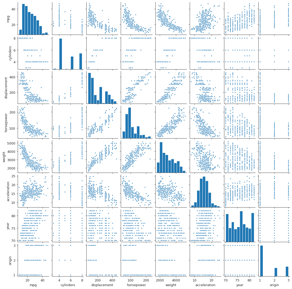
Scatter plot matrix of `Auto` data set

plt.close("all")
spm = sns.pairplot(auto, plot_kws = {'s': 10})
spm.fig.set_size_inches(12, 12)
spm.savefig("img/3_auto_scatter.png", dpi=90)

Correlation matrix

I find heat maps to be better for visualizing correlation matrices than tables. Since the correlation matrix is symmetric we can ignore either of the lower or the upper triangles. We can also ignore the diagonal since it is always going to be 1.

corr_mat = auto[auto.columns[:-1]].corr()

plt.close("all")
fig, ax = plt.subplots()

# Custom diverging color map.
cmap = sns.diverging_palette(220, 10, sep=80, n=7)

# Mask for upper triangle.
mask = np.triu(np.ones_like(corr_mat, dtype=np.bool))

with sns.axes_style("white"):
    sns.heatmap(corr_mat, mask=mask, cmap=cmap, annot=True, robust=True, ax=ax)

fig.savefig("img/3_auto_corr_heat.png")

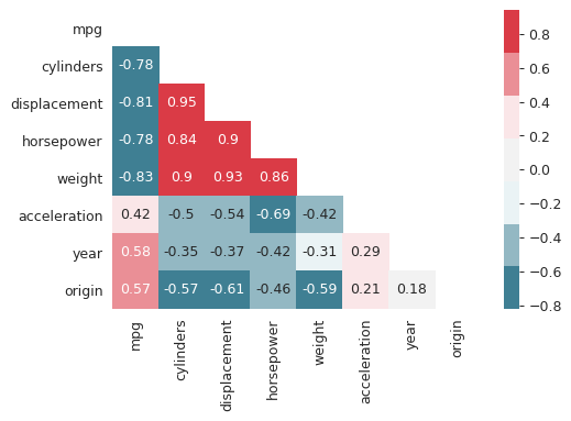
We see that mpg has considerable negative correlations with cylinders, displacement, horsepower, and weight. This matches what we saw in the scatter plot matrix above. Similarly cylinders, displacement, horsepower and weight are all correlated with each other.

Multiple linear regression with `Auto` data set

We could do this with the statsmodels.formula API but that involves more typing, so we will use the statsmodels API.

import statsmodels.api as sm

Y = auto["mpg"]
X = auto[auto.columns[1:-1]]
X = sm.add_constant(X) # For the intercept.
ml_model = sm.OLS(Y, X).fit()
print(ml_model.summary())

                            OLS Regression Results
==============================================================================
Dep. Variable:                    mpg   R-squared:                       0.821
Model:                            OLS   Adj. R-squared:                  0.818
Method:                 Least Squares   F-statistic:                     252.4
Date:                Mon, 25 May 2020   Prob (F-statistic):          2.04e-139
Time:                        17:25:25   Log-Likelihood:                -1023.5
No. Observations:                 392   AIC:                             2063.
Df Residuals:                     384   BIC:                             2095.
Df Model:                           7
Covariance Type:            nonrobust
================================================================================
                   coef    std err          t      P>|t|      [0.025      0.975]
--------------------------------------------------------------------------------
const          -17.2184      4.644     -3.707      0.000     -26.350      -8.087
cylinders       -0.4934      0.323     -1.526      0.128      -1.129       0.142
displacement     0.0199      0.008      2.647      0.008       0.005       0.035
horsepower      -0.0170      0.014     -1.230      0.220      -0.044       0.010
weight          -0.0065      0.001     -9.929      0.000      -0.008      -0.005
acceleration     0.0806      0.099      0.815      0.415      -0.114       0.275
year             0.7508      0.051     14.729      0.000       0.651       0.851
origin           1.4261      0.278      5.127      0.000       0.879       1.973
==============================================================================
Omnibus:                       31.906   Durbin-Watson:                   1.309
Prob(Omnibus):                  0.000   Jarque-Bera (JB):               53.100
Skew:                           0.529   Prob(JB):                     2.95e-12
Kurtosis:                       4.460   Cond. No.                     8.59e+04
==============================================================================

Warnings:
[1] Standard Errors assume that the covariance matrix of the errors is correctly specified.
[2] The condition number is large, 8.59e+04. This might indicate that there are
strong multicollinearity or other numerical problems.

The large F-statistic indicates that we can ignore the null hypothesis, which says that the response mpg does not depend on the predictors. The probability that this data could be generated if the null hypothesis was true is essentially zero (2.04E-139).
Looking at the p-values of the individual predictors we see that weight, year, and origin have the most statistically significant relation with mpg. We can also argue that displacement has a somewhat significant relation with mpg. On the other hand cylinders, horsepower, and acceleration do not have a significant statistical relationship. This is not necessarily surprising. Given the correlation between mpg, displacement, cylinders and horsepower I think one can argue that the information in cylinders and horsepower is redundant.
The coefficient for the year variable suggests that every year the mpg increases by 0.7508, i.e. the cars become more fuel-efficient every year.

Diagnostic plots

We make the same diagnostic plots as the previous exercise.

Residuals vs Fitted plot

fitted_vals = ml_model.fittedvalues

plt.close("all")
fig, ax = plt.subplots()
residplot = sns.residplot(x=fitted_vals, y="mpg", data=auto,
                          lowess=True,
                          line_kws={"color": "red"},
                          ax=ax)
ax.set_xlabel("Fitted values")
ax.set_ylabel("Residuals")
sns.despine()
fig.savefig("img/3_ml_res_vs_fit.png", dpi=90)

This plot clearly shows that there is non-linearity in the data.

Normal Q-Q plot

import statsmodels.api as sm

residuals = ml_model.resid

plt.close("all")
fig, ax = plt.subplots()
qqplot = sm.qqplot(residuals, line='45', ax=ax, fit=True)
ax.set_ylabel("Standardized Residuals")
sns.despine()
fig.savefig("img/3_ml_auto_qq.png", dpi=90)

Though there are some points that are far from the $45^\circ$ fitted line, most of the points lie close to the line, indicating that the residuals are mostly normally distributed.

Scale-Location plot

# normalized residuals and their square roots
norm_residuals = ml_model.get_influence().resid_studentized_internal
norm_residuals_abs_sqrt = np.sqrt(np.abs(norm_residuals))

plt.close("all")
fig, ax = plt.subplots()
slplot = sns.regplot(fitted_vals, norm_residuals_abs_sqrt,
                     lowess=True,
                     line_kws={"color" : "red"},
                     ax=ax)
ax.set_xlabel("Fitted values")
ax.set_ylabel("Sqrt of |Standardized Residuals|")
sns.despine()
fig.savefig("img/3_ml_auto_scale_loc.png", dpi=90)

The variance in the standardized residuals is less as compared to the single regression plot, but there is still quite a bit of variance, which means homoscedasticity is not held.

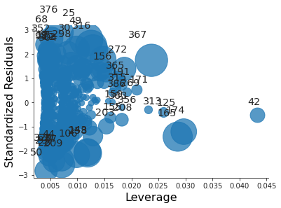
Residuals vs Leverage plot

plt.close("all")
fig, ax = plt.subplots()
rlplot = sm.graphics.influence_plot(ml_model, criterion="Cooks", ax=ax)
sns.despine()
ax.set_xlabel("Leverage")
ax.set_ylabel("Standardized Residuals")
ax.set_title(" ")
fig.savefig("img/3_ml_auto_res_vs_lev.png", dpi=90)

Point 13 has a high leverage but not a very high residual.

Interaction effects

We go back to the statsmodels.formula API. Additionally I will drop cylinders, horsepower, and acceleration from the model. I will try the following interaction terms:

year : origin : this will add a new predictor which is a product of year and origin, but will not include year and origin separately,
year * origin : this will add the product of year and origin, but also include year and origin separately,
year * weight : same as the above, except for weight in place of origin.

ml_model_1 = smf.ols(formula="mpg ~ displacement + weight + year : origin",
                     data=auto).fit()
ml_model_2 = smf.ols(formula="mpg ~ displacement + weight + year * origin",
                     data=auto).fit()
ml_model_3 = smf.ols(formula="mpg ~ displacement + weight * year + origin",
                     data=auto).fit()

Summary of first interaction model

print(ml_model_1.summary())

                            OLS Regression Results
==============================================================================
Dep. Variable:                    mpg   R-squared:                       0.714
Model:                            OLS   Adj. R-squared:                  0.712
Method:                 Least Squares   F-statistic:                     322.7
Date:                Mon, 25 May 2020   Prob (F-statistic):          4.85e-105
Time:                        18:13:04   Log-Likelihood:                -1115.9
No. Observations:                 392   AIC:                             2240.
Df Residuals:                     388   BIC:                             2256.
Df Model:                           3
Covariance Type:            nonrobust
================================================================================
                   coef    std err          t      P>|t|      [0.025      0.975]
--------------------------------------------------------------------------------
Intercept       39.8822      1.427     27.939      0.000      37.076      42.689
displacement    -0.0100      0.006     -1.728      0.085      -0.021       0.001
weight          -0.0056      0.001     -8.137      0.000      -0.007      -0.004
year:origin      0.0193      0.004      4.502      0.000       0.011       0.028
==============================================================================
Omnibus:                       41.720   Durbin-Watson:                   0.883
Prob(Omnibus):                  0.000   Jarque-Bera (JB):               68.034
Skew:                           0.674   Prob(JB):                     1.69e-15
Kurtosis:                       4.532   Cond. No.                     2.09e+04
==============================================================================

Warnings:
[1] Standard Errors assume that the covariance matrix of the errors is correctly specified.
[2] The condition number is large, 2.09e+04. This might indicate that there are
strong multicollinearity or other numerical problems.

The large F-statistic invalidates the null hypothesis. The individual p-values show that displacement is not really significant, but the product of year and origin is. Additionally the $R^2$ value tells us that this model explains around 71% of the mpg values.

Summary of second interaction model

print(ml_model_2.summary())

                            OLS Regression Results
==============================================================================
Dep. Variable:                    mpg   R-squared:                       0.823
Model:                            OLS   Adj. R-squared:                  0.821
Method:                 Least Squares   F-statistic:                     359.5
Date:                Mon, 25 May 2020   Prob (F-statistic):          8.65e-143
Time:                        18:17:24   Log-Likelihood:                -1021.6
No. Observations:                 392   AIC:                             2055.
Df Residuals:                     386   BIC:                             2079.
Df Model:                           5
Covariance Type:            nonrobust
================================================================================
                   coef    std err          t      P>|t|      [0.025      0.975]
--------------------------------------------------------------------------------
Intercept        7.9270      8.873      0.893      0.372      -9.519      25.373
displacement     0.0016      0.005      0.319      0.750      -0.008       0.011
weight          -0.0064      0.001    -11.571      0.000      -0.007      -0.005
year             0.4313      0.113      3.818      0.000       0.209       0.653
origin         -14.4936      4.707     -3.079      0.002     -23.749      -5.239
year:origin      0.2023      0.060      3.345      0.001       0.083       0.321
==============================================================================
Omnibus:                       38.636   Durbin-Watson:                   1.322
Prob(Omnibus):                  0.000   Jarque-Bera (JB):               71.804
Skew:                           0.584   Prob(JB):                     2.56e-16
Kurtosis:                       4.741   Cond. No.                     1.84e+05
==============================================================================

Warnings:
[1] Standard Errors assume that the covariance matrix of the errors is correctly specified.
[2] The condition number is large, 1.84e+05. This might indicate that there are
strong multicollinearity or other numerical problems.

The $R^2$ value has increased; it is now almost the same as the $R^2$ value for the model with all the quantitative predictors but no interaction. This model explains around 82% of the mpg values. Additionally we see that year is more significant than origin or the product of year and origin. Also, in addition to displacement, the intercept term appears to be insignificant too.

Summary of third interaction model

print(ml_model_3.summary())

                            OLS Regression Results
==============================================================================
Dep. Variable:                    mpg   R-squared:                       0.840
Model:                            OLS   Adj. R-squared:                  0.838
Method:                 Least Squares   F-statistic:                     404.4
Date:                Mon, 25 May 2020   Prob (F-statistic):          5.53e-151
Time:                        18:22:57   Log-Likelihood:                -1002.4
No. Observations:                 392   AIC:                             2017.
Df Residuals:                     386   BIC:                             2041.
Df Model:                           5
Covariance Type:            nonrobust
================================================================================
                   coef    std err          t      P>|t|      [0.025      0.975]
--------------------------------------------------------------------------------
Intercept     -107.6004     12.904     -8.339      0.000    -132.971     -82.229
displacement    -0.0004      0.005     -0.088      0.930      -0.009       0.009
weight           0.0260      0.005      5.722      0.000       0.017       0.035
year             1.9624      0.172     11.436      0.000       1.625       2.300
weight:year     -0.0004   5.97e-05     -7.214      0.000      -0.001      -0.000
origin           0.9116      0.255      3.579      0.000       0.411       1.412
==============================================================================
Omnibus:                       43.792   Durbin-Watson:                   1.372
Prob(Omnibus):                  0.000   Jarque-Bera (JB):               89.759
Skew:                           0.619   Prob(JB):                     3.23e-20
Kurtosis:                       4.991   Cond. No.                     1.90e+07
==============================================================================

Warnings:
[1] Standard Errors assume that the covariance matrix of the errors is correctly specified.
[2] The condition number is large, 1.9e+07. This might indicate that there are
strong multicollinearity or other numerical problems.

The $R^2$ increased a bit, and it appears other than displacement all the other predictors are significant.

Interaction model with two interactions

We will try an additional model with two interactions: displacement * weight and weight * year.

ml_model_4 = smf.ols("mpg ~ displacement * weight + weight * year + origin",
                     data=auto).fit()
print(ml_model_4.summary())

                            OLS Regression Results
==============================================================================
Dep. Variable:                    mpg   R-squared:                       0.859
Model:                            OLS   Adj. R-squared:                  0.856
Method:                 Least Squares   F-statistic:                     389.6
Date:                Mon, 25 May 2020   Prob (F-statistic):          4.10e-160
Time:                        18:33:39   Log-Likelihood:                -977.80
No. Observations:                 392   AIC:                             1970.
Df Residuals:                     385   BIC:                             1997.
Df Model:                           6
Covariance Type:            nonrobust
=======================================================================================
                          coef    std err          t      P>|t|      [0.025      0.975]
---------------------------------------------------------------------------------------
Intercept             -61.3985     13.741     -4.468      0.000     -88.416     -34.381
displacement           -0.0604      0.009     -6.424      0.000      -0.079      -0.042
weight                  0.0090      0.005      1.848      0.065      -0.001       0.019
displacement:weight  1.708e-05   2.38e-06      7.169      0.000    1.24e-05    2.18e-05
year                    1.4982      0.174      8.616      0.000       1.156       1.840
weight:year            -0.0002   6.16e-05     -4.037      0.000      -0.000      -0.000
origin                  0.3388      0.253      1.342      0.181      -0.158       0.835
==============================================================================
Omnibus:                       62.892   Durbin-Watson:                   1.412
Prob(Omnibus):                  0.000   Jarque-Bera (JB):              174.597
Skew:                           0.754   Prob(JB):                     1.22e-38
Kurtosis:                       5.901   Cond. No.                     8.00e+07
==============================================================================

Warnings:
[1] Standard Errors assume that the covariance matrix of the errors is correctly specified.
[2] The condition number is large,  8e+07. This might indicate that there are
strong multicollinearity or other numerical problems.

This is interesting. We see that the $R^2$ value has increased further, but now displacement has become significant whereas weight and origin have become relatively insignificant. The interaction terms are still significant. My understanding of this model is that while weight does not directly affect mpg, it increases displacement, and that affects the mpg.

Models with variable transformations

ml_model_trans = smf.ols(formula="mpg ~ np.log(weight) + np.power(weight, 2) + year",
                         data=auto).fit()
print(ml_model_trans.summary())

                            OLS Regression Results
==============================================================================
Dep. Variable:                    mpg   R-squared:                       0.851
Model:                            OLS   Adj. R-squared:                  0.850
Method:                 Least Squares   F-statistic:                     749.0
Date:                Mon, 25 May 2020   Prob (F-statistic):          4.19e-162
Time:                        18:49:50   Log-Likelihood:                -1001.5
No. Observations:                 397   AIC:                             2011.
Df Residuals:                     393   BIC:                             2027.
Df Model:                           3
Covariance Type:            nonrobust
=======================================================================================
                          coef    std err          t      P>|t|      [0.025      0.975]
---------------------------------------------------------------------------------------
Intercept             213.1803     16.063     13.271      0.000     181.599     244.761
np.log(weight)        -32.5971      2.150    -15.159      0.000     -36.825     -28.369
np.power(weight, 2)  6.506e-07   1.12e-07      5.804      0.000     4.3e-07    8.71e-07
year                    0.8355      0.044     19.023      0.000       0.749       0.922
==============================================================================
Omnibus:                       69.088   Durbin-Watson:                   1.361
Prob(Omnibus):                  0.000   Jarque-Bera (JB):              168.823
Skew:                           0.864   Prob(JB):                     2.19e-37
Kurtosis:                       5.687   Cond. No.                     1.17e+09
==============================================================================

Warnings:
[1] Standard Errors assume that the covariance matrix of the errors is correctly specified.
[2] The condition number is large, 1.17e+09. This might indicate that there are
strong multicollinearity or other numerical problems.

The F-statistic and the p-values indicate that these transformations are statistically significant.

Question 10

Multiple regression with `Carseats` data set

So far I had been loading the data sets from local .csv files, but I recently found out that statsmodels makes them automatically available using the Rdatasets project. So going forward I will be using that whenever possible.

import statsmodels.api as sm

carseats = sm.datasets.get_rdataset("Carseats", package="ISLR")
print(carseats.__doc__)

+----------+-----------------+
| Carseats | R Documentation |
+----------+-----------------+

Sales of Child Car Seats
------------------------

Description
~~~~~~~~~~~

A simulated data set containing sales of child car seats at 400
different stores.

Usage
~~~~~

::

   Carseats

Format
~~~~~~

A data frame with 400 observations on the following 11 variables.

``Sales``
   Unit sales (in thousands) at each location

``CompPrice``
   Price charged by competitor at each location

``Income``
   Community income level (in thousands of dollars)

``Advertising``
   Local advertising budget for company at each location (in thousands
   of dollars)

``Population``
   Population size in region (in thousands)

``Price``
   Price company charges for car seats at each site

``ShelveLoc``
   A factor with levels ``Bad``, ``Good`` and ``Medium`` indicating the
   quality of the shelving location for the car seats at each site

``Age``
   Average age of the local population

``Education``
   Education level at each location

``Urban``
   A factor with levels ``No`` and ``Yes`` to indicate whether the store
   is in an urban or rural location

``US``
   A factor with levels ``No`` and ``Yes`` to indicate whether the store
   is in the US or not

Source
~~~~~~

Simulated data

References
~~~~~~~~~~

James, G., Witten, D., Hastie, T., and Tibshirani, R. (2013) *An
Introduction to Statistical Learning with applications in R*,
`www.StatLearning.com <www.StatLearning.com>`__, Springer-Verlag, New
York

Examples
~~~~~~~~

::

   summary(Carseats)
   lm.fit=lm(Sales~Advertising+Price,data=Carseats)

Multiple linear regression to predict Sales using Price, Urban, and US.

import statsmodels.formula.api as smf

model = smf.ols(formula="Sales ~ Price + Urban + US",
                data=carseats.data).fit()

print(model.summary())

                            OLS Regression Results
==============================================================================
Dep. Variable:                  Sales   R-squared:                       0.239
Model:                            OLS   Adj. R-squared:                  0.234
Method:                 Least Squares   F-statistic:                     41.52
Date:                Thu, 28 May 2020   Prob (F-statistic):           2.39e-23
Time:                        18:21:58   Log-Likelihood:                -927.66
No. Observations:                 400   AIC:                             1863.
Df Residuals:                     396   BIC:                             1879.
Df Model:                           3
Covariance Type:            nonrobust
================================================================================
                   coef    std err          t      P>|t|      [0.025      0.975]
--------------------------------------------------------------------------------
Intercept       13.0435      0.651     20.036      0.000      11.764      14.323
Urban[T.Yes]    -0.0219      0.272     -0.081      0.936      -0.556       0.512
US[T.Yes]        1.2006      0.259      4.635      0.000       0.691       1.710
Price           -0.0545      0.005    -10.389      0.000      -0.065      -0.044
==============================================================================
Omnibus:                        0.676   Durbin-Watson:                   1.912
Prob(Omnibus):                  0.713   Jarque-Bera (JB):                0.758
Skew:                           0.093   Prob(JB):                        0.684
Kurtosis:                       2.897   Cond. No.                         628.
==============================================================================

Warnings:
[1] Standard Errors assume that the covariance matrix of the errors is correctly specified.

The F-statistic is larger than 1, though much smaller compared to the F-statistics in the last problem. I think this means that the alternative hypothesis is viable, but not completely sure about that.

From the individual p-values we can conclude that Urban is not a statistically significant predictor for Sales.

Interpretation of coefficient of predictors

Since Urban is not a statistically significant predictor we do not need to worry about its coefficient. The coefficient for US indicates that if the store is in the US then it then the sales will increase by about 1200 units. On the other hand the coefficient for Price says that an increase in price will result in a decrease in sales.

Linear model equation

The equation for this model is

\begin{align} Y = 13.04 - 0.02 X_1 + 1.20 X_2 - 0.05 X_3, \end{align}

where $Y$, $X_1$, $X_2$, and $X_3$ stand for Sales, Urban, US, and Price, respectively. $X_1 = 1$ if the store is an urban location, and $0$ otherwise. Similarly $X_2 = 1$ if the store is in the US, and $0$ if it is not.

Null hypothesis rejection

We can reject the null hypothesis for US, and Price, since the associated p-values are effectively 0.

Smaller multiple linear model for `Carseats` sales

small_model = smf.ols(formula="Sales ~ US + Price", data=carseats.data).fit()
print(small_model.summary())

                            OLS Regression Results
==============================================================================
Dep. Variable:                  Sales   R-squared:                       0.239
Model:                            OLS   Adj. R-squared:                  0.235
Method:                 Least Squares   F-statistic:                     62.43
Date:                Thu, 28 May 2020   Prob (F-statistic):           2.66e-24
Time:                        18:45:15   Log-Likelihood:                -927.66
No. Observations:                 400   AIC:                             1861.
Df Residuals:                     397   BIC:                             1873.
Df Model:                           2
Covariance Type:            nonrobust
==============================================================================
                 coef    std err          t      P>|t|      [0.025      0.975]
------------------------------------------------------------------------------
Intercept     13.0308      0.631     20.652      0.000      11.790      14.271
US[T.Yes]      1.1996      0.258      4.641      0.000       0.692       1.708
Price         -0.0545      0.005    -10.416      0.000      -0.065      -0.044
==============================================================================
Omnibus:                        0.666   Durbin-Watson:                   1.912
Prob(Omnibus):                  0.717   Jarque-Bera (JB):                0.749
Skew:                           0.092   Prob(JB):                        0.688
Kurtosis:                       2.895   Cond. No.                         607.
==============================================================================

Warnings:
[1] Standard Errors assume that the covariance matrix of the errors is correctly specified.

Based on the $R^2$ values both the models fit the data similarly.

Confidence intervals of fitted parameters

print(small_model.conf_int())

                  0          1
Intercept  11.79032  14.271265
US[T.Yes]   0.69152   1.707766
Price      -0.06476  -0.044195

The confidence intervals are also printed in the summary, but this is probably more convenient.

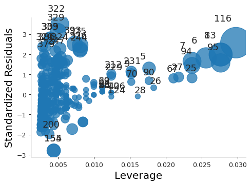
Outliers and leverages

To see if there are any leverage points we need to first calculate the average leverage, $(p + 1) / n$, for the data.

npredictors = 2
nobservations = len(carseats.data)
avg_leverage = (npredictors + 1) / nobservations

print(f"Average leverage: {avg_leverage}")

Average leverage: 0.0075

The Residuals vs Leverage plot is the easiest way to check for outliers and high leverage observations.

import matplotlib.pyplot as plt
import seaborn as sns

sns.set_style("ticks")

plt.close("all")
fig, ax = plt.subplots()
rlplot = sm.graphics.influence_plot(small_model, criterion="Cooks", ax=ax)
sns.despine()
ax.set_xlabel("Leverage")
ax.set_ylabel("Standardized Residuals")
ax.set_title(" ")
fig.savefig("img/3.10.h_res_vs_lev.png", dpi=90)

3.10.h_res_vs_lev.png

All the residuals are between -3 and 3, so there are no outliers. However there are a lot of points whose leverage greatly exceeds the average leverage. Thus there are high leverage observations.

Question 11

Simple linear regression with synthetic data

import pandas as pd
import numpy as np
import matplotlib.pyplot as plt
import seaborn as sns

sns.set_style("ticks")

rng = np.random.default_rng(seed=42)
x = rng.normal(size=100)
y = 2 * x + rng.normal(size=100)

data = pd.DataFrame({"X" : x, "Y" : y})

plt.close("all")
fig, ax = plt.subplots()
sp = sns.scatterplot(x="X", y="Y", data=data, ax=ax)
sns.despine()
fig.savefig("img/3.11.a_data.png", dpi=90)

3.11.a_data.png

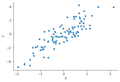
Now we do a simple linear regression with this synthetic data. This model will not have an intercept: $Y = βX$.

import statsmodels.formula.api as smf

model = smf.ols("Y ~ X - 1", data=data).fit()
print(model.summary())

                                 OLS Regression Results
=======================================================================================
Dep. Variable:                      Y   R-squared (uncentered):                   0.741
Model:                            OLS   Adj. R-squared (uncentered):              0.738
Method:                 Least Squares   F-statistic:                              283.3
Date:                Fri, 29 May 2020   Prob (F-statistic):                    8.30e-31
Time:                        07:28:26   Log-Likelihood:                         -138.87
No. Observations:                 100   AIC:                                      279.7
Df Residuals:                      99   BIC:                                      282.4
Df Model:                           1
Covariance Type:            nonrobust
==============================================================================
                 coef    std err          t      P>|t|      [0.025      0.975]
------------------------------------------------------------------------------
X              2.1196      0.126     16.833      0.000       1.870       2.369
==============================================================================
Omnibus:                        2.995   Durbin-Watson:                   1.681
Prob(Omnibus):                  0.224   Jarque-Bera (JB):                2.970
Skew:                           0.408   Prob(JB):                        0.227
Kurtosis:                       2.787   Cond. No.                         1.00
==============================================================================

Warnings:
[1] Standard Errors assume that the covariance matrix of the errors is correctly specified.

The coefficient estimate is $\hat{β} = 2.1196$ with a standard error of $0.126$. The t-statistic is 16.833 and the associated p-value is 0. This means we can reject the null hypothesis.

Inverse simple linear relation with synthetic data

We are going to use the same data, but now with X as the response and Y as the predictor.

model2 = smf.ols("X ~ Y - 1", data=data).fit()
print(model2.summary())

                                 OLS Regression Results
=======================================================================================
Dep. Variable:                      X   R-squared (uncentered):                   0.741
Model:                            OLS   Adj. R-squared (uncentered):              0.738
Method:                 Least Squares   F-statistic:                              283.3
Date:                Fri, 29 May 2020   Prob (F-statistic):                    8.30e-31
Time:                        07:36:14   Log-Likelihood:                         -48.770
No. Observations:                 100   AIC:                                      99.54
Df Residuals:                      99   BIC:                                      102.1
Df Model:                           1
Covariance Type:            nonrobust
==============================================================================
                 coef    std err          t      P>|t|      [0.025      0.975]
------------------------------------------------------------------------------
Y              0.3496      0.021     16.833      0.000       0.308       0.391
==============================================================================
Omnibus:                        1.369   Durbin-Watson:                   1.557
Prob(Omnibus):                  0.504   Jarque-Bera (JB):                1.145
Skew:                          -0.020   Prob(JB):                        0.564
Kurtosis:                       2.477   Cond. No.                         1.00
==============================================================================

Warnings:
[1] Standard Errors assume that the covariance matrix of the errors is correctly specified.

The coefficient estimate is $\hat{β} = 0.3496$ with a standard error of $0.021$. The t-statistic is $16.833$ and the associated p-value is 0. This means we can reject the null hypothesis.

Relation between the two regressions

Given the underlying true model we should have expected that the coefficients of the two models would be multiplicative inverses of each other. But they are not. The reason being that the two models are minimizing different residual sum of squares. For the two models the residual sum of squares are

\begin{align} \mathrm{RSS}^{(1)} &= ∑_{i=1}^n (y_i - \hat{β}^(1) x_i)^2, \\ \mathrm{RSS}^{(2)} &= ∑_{i=1}^n (x_i - \hat{β}^(2) y_i)^2, \end{align}

respectively. $\mathrm{RSS}^(1)$ is minimized when $\hat{β}^(1) = ∑y_i x_i / ∑ x_i^2$, and $\mathrm{RSS}^(2)$ is minimized when $\hat{β}^(2) = ∑x_i y_i / ∑ y_i^2$. If $\hat{β}^(1) = 1 / \hat{β}^(2)$ then we have

\begin{align} (∑_{i=1}^n x_i y_i)^2 = ∑_{i=1}^n x_i^2 ∑_{i=1}^n y_i^2. \end{align}

Since here $X$ and $Y$ are random variables with zero mean we can interpret the above equation as

\begin{align} \mathrm{Cov}(X, Y) = \mathrm{Var}(X) \mathrm{Var}(Y). \end{align}

This is true only if the true relation is $y_i = β x_i + γ$ for some nonzero constants $β$ and $γ$ (See DeGroot and Schervish, Theorem 4.6.3, or ProofWiki for a proof of this statement.). But the true relation in this case was $y_i = β x_i + ϵ$, where $ϵ$ is a Gaussian random variable with zero mean. Thus the above statement is not true, and hence $\hat{β}^(1) ≠ 1 / \hat{β}^(2)$. For a more detailed discussion on this check Stats StackExchange.

t-statistic for first model

The t-statistic for a simple linear fit without intercept is $\hat{β} / \mathrm{SE}(\hat{β})$ where $\hat{β} = ∑_i x_i y_i / ∑_i x_i^2$, and the standard error is

\begin{align} \mathrm{SE}(\hat{β} = \frac{\sqrt{∑_i (y_i - x_i \hat{β})^2}}{(n-1) ∑_i x_i^2}. \end{align}

Substituting the expression for $\hat{β}$ in to the expressions for the standard error and the t-statistic gives us the expected expression for the t-statistic. The trick is to realize that the summation indices are dummy variables, i.e. $∑_{i=1}^n x_i^2 = ∑_{j=1}^n x_j^2$. Numerically we can conform this as follows:

n = len(data)
x, y = data["X"], data["Y"]
t = (np.sqrt(n - 1) * np.sum(x * y)
     / np.sqrt(np.sum(x ** 2) * np.sum(y ** 2) - np.sum(x * y) ** 2))
print(f"t-statistic: {t:.3f}")

t-statistic: 16.833

t-statistic for second model

The expression for the t-statistic is symmetric in $X$ and $Y$, so irrespective of whether we are regressing $Y$ onto $X$ or $X$ onto $Y$, we will have the same t-statistic.

t-statistic for models with intercept

model3 = smf.ols(formula="Y ~ X", data=data).fit()
model4 = smf.ols(formula="X ~ Y", data=data).fit()

print(model3.summary())

                            OLS Regression Results
==============================================================================
Dep. Variable:                      Y   R-squared:                       0.740
Model:                            OLS   Adj. R-squared:                  0.738
Method:                 Least Squares   F-statistic:                     279.2
Date:                Sat, 30 May 2020   Prob (F-statistic):           1.94e-30
Time:                        00:26:31   Log-Likelihood:                -138.87
No. Observations:                 100   AIC:                             281.7
Df Residuals:                      98   BIC:                             287.0
Df Model:                           1
Covariance Type:            nonrobust
==============================================================================
                 coef    std err          t      P>|t|      [0.025      0.975]
------------------------------------------------------------------------------
Intercept     -0.0046      0.098     -0.047      0.962      -0.200       0.190
X              2.1192      0.127     16.709      0.000       1.867       2.371
==============================================================================
Omnibus:                        2.996   Durbin-Watson:                   1.682
Prob(Omnibus):                  0.224   Jarque-Bera (JB):                2.971
Skew:                           0.409   Prob(JB):                        0.226
Kurtosis:                       2.787   Cond. No.                         1.30
==============================================================================

Warnings:
[1] Standard Errors assume that the covariance matrix of the errors is correctly specified.

print(model4.summary())

                            OLS Regression Results
==============================================================================
Dep. Variable:                      X   R-squared:                       0.740
Model:                            OLS   Adj. R-squared:                  0.738
Method:                 Least Squares   F-statistic:                     279.2
Date:                Sat, 30 May 2020   Prob (F-statistic):           1.94e-30
Time:                        00:26:47   Log-Likelihood:                -48.728
No. Observations:                 100   AIC:                             101.5
Df Residuals:                      98   BIC:                             106.7
Df Model:                           1
Covariance Type:            nonrobust
==============================================================================
                 coef    std err          t      P>|t|      [0.025      0.975]
------------------------------------------------------------------------------
Intercept     -0.0114      0.040     -0.287      0.775      -0.091       0.068
Y              0.3493      0.021     16.709      0.000       0.308       0.391
==============================================================================
Omnibus:                        1.373   Durbin-Watson:                   1.559
Prob(Omnibus):                  0.503   Jarque-Bera (JB):                1.146
Skew:                          -0.018   Prob(JB):                        0.564
Kurtosis:                       2.477   Cond. No.                         1.91
==============================================================================

Warnings:
[1] Standard Errors assume that the covariance matrix of the errors is correctly specified.

We can see that the t-coefficient for the predictors is same for both models.

Question 12

Equal regression coefficients

As this is a regression without intercept we can use the expressions derived in the previous question. The coefficients will be same when $∑_i x_i^2 = ∑_i y_i^2$. This is particularly true when $X = Y$.

Different coefficient estimates - numerical

Essentially reusing question 11.

rng = np.random.default_rng(seed=42)
x = rng.normal(size=100)
y = 2 * x + rng.normal(size=100)

data = pd.DataFrame({"X" : x, "Y" : y})

plt.close("all")
fig, ax = plt.subplots()
sp = sns.scatterplot(x="X", y="Y", data=data, ax=ax)
sns.despine()
fig.savefig("img/3.12.b_data.png", dpi=90)

3.12.b_data.png

model1 = smf.ols("Y ~ X - 1", data=data).fit()
model2 = smf.ols("X ~ Y - 1", data=data).fit()

print(model1.summary())

                                 OLS Regression Results
=======================================================================================
Dep. Variable:                      Y   R-squared (uncentered):                   0.741
Model:                            OLS   Adj. R-squared (uncentered):              0.738
Method:                 Least Squares   F-statistic:                              283.3
Date:                Sat, 30 May 2020   Prob (F-statistic):                    8.30e-31
Time:                        00:47:09   Log-Likelihood:                         -138.87
No. Observations:                 100   AIC:                                      279.7
Df Residuals:                      99   BIC:                                      282.4
Df Model:                           1
Covariance Type:            nonrobust
==============================================================================
                 coef    std err          t      P>|t|      [0.025      0.975]
------------------------------------------------------------------------------
X              2.1196      0.126     16.833      0.000       1.870       2.369
==============================================================================
Omnibus:                        2.995   Durbin-Watson:                   1.681
Prob(Omnibus):                  0.224   Jarque-Bera (JB):                2.970
Skew:                           0.408   Prob(JB):                        0.227
Kurtosis:                       2.787   Cond. No.                         1.00
==============================================================================

Warnings:
[1] Standard Errors assume that the covariance matrix of the errors is correctly specified.

print(model2.summary())

                                 OLS Regression Results
=======================================================================================
Dep. Variable:                      X   R-squared (uncentered):                   0.741
Model:                            OLS   Adj. R-squared (uncentered):              0.738
Method:                 Least Squares   F-statistic:                              283.3
Date:                Sat, 30 May 2020   Prob (F-statistic):                    8.30e-31
Time:                        00:47:17   Log-Likelihood:                         -48.770
No. Observations:                 100   AIC:                                      99.54
Df Residuals:                      99   BIC:                                      102.1
Df Model:                           1
Covariance Type:            nonrobust
==============================================================================
                 coef    std err          t      P>|t|      [0.025      0.975]
------------------------------------------------------------------------------
Y              0.3496      0.021     16.833      0.000       0.308       0.391
==============================================================================
Omnibus:                        1.369   Durbin-Watson:                   1.557
Prob(Omnibus):                  0.504   Jarque-Bera (JB):                1.145
Skew:                          -0.020   Prob(JB):                        0.564
Kurtosis:                       2.477   Cond. No.                         1.00
==============================================================================

Warnings:
[1] Standard Errors assume that the covariance matrix of the errors is correctly specified.

Same coefficient estimates - numerical

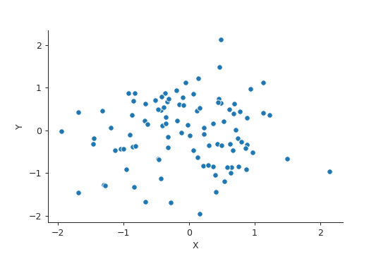
We need $∑_i x_i^2 = ∑_i y_i^2$. Setting $X = Y$ works, but $Y = \mathrm{Permutation}(X)$ would work too, and is more general.

rng = np.random.default_rng(seed=42)
x = rng.normal(size=100)
y = np.random.permutation(x)

data = pd.DataFrame({"X" : x, "Y" : y})

plt.close("all")
fig, ax = plt.subplots()
sp = sns.scatterplot(x="X", y="Y", data=data, ax=ax)
sns.despine()
fig.savefig("img/3.12.b_data.png", dpi=90)

model3 = smf.ols("Y ~ X - 1", data=data).fit()
model4 = smf.ols("X ~ Y - 1", data=data).fit()

print(model3.summary())

                                 OLS Regression Results
=======================================================================================
Dep. Variable:                      Y   R-squared (uncentered):                   0.002
Model:                            OLS   Adj. R-squared (uncentered):             -0.008
Method:                 Least Squares   F-statistic:                             0.2018
Date:                Sat, 30 May 2020   Prob (F-statistic):                       0.654
Time:                        00:52:14   Log-Likelihood:                         -116.23
No. Observations:                 100   AIC:                                      234.5
Df Residuals:                      99   BIC:                                      237.1
Df Model:                           1
Covariance Type:            nonrobust
==============================================================================
                 coef    std err          t      P>|t|      [0.025      0.975]
------------------------------------------------------------------------------
X              0.0451      0.100      0.449      0.654      -0.154       0.244
==============================================================================
Omnibus:                        0.651   Durbin-Watson:                   1.772
Prob(Omnibus):                  0.722   Jarque-Bera (JB):                0.787
Skew:                          -0.142   Prob(JB):                        0.675
Kurtosis:                       2.671   Cond. No.                         1.00
==============================================================================

Warnings:
[1] Standard Errors assume that the covariance matrix of the errors is correctly specified.

print(model4.summary())

                                 OLS Regression Results
=======================================================================================
Dep. Variable:                      X   R-squared (uncentered):                   0.002
Model:                            OLS   Adj. R-squared (uncentered):             -0.008
Method:                 Least Squares   F-statistic:                             0.2018
Date:                Sat, 30 May 2020   Prob (F-statistic):                       0.654
Time:                        00:52:20   Log-Likelihood:                         -116.23
No. Observations:                 100   AIC:                                      234.5
Df Residuals:                      99   BIC:                                      237.1
Df Model:                           1
Covariance Type:            nonrobust
==============================================================================
                 coef    std err          t      P>|t|      [0.025      0.975]
------------------------------------------------------------------------------
Y              0.0451      0.100      0.449      0.654      -0.154       0.244
==============================================================================
Omnibus:                        0.296   Durbin-Watson:                   1.833
Prob(Omnibus):                  0.862   Jarque-Bera (JB):                0.446
Skew:                          -0.105   Prob(JB):                        0.800
Kurtosis:                       2.749   Cond. No.                         1.00
==============================================================================

Warnings:
[1] Standard Errors assume that the covariance matrix of the errors is correctly specified.

Question 13

Feature vector

rng = np.random.default_rng(seed=42)
x = rng.normal(loc=0, scale=1, size=100)

Error vector

eps = rng.normal(loc=0, scale=0.25, size=100)

Response vector

y = -1 + 0.5 * x + eps

The length of y is 100, and $β_0 = -1$, and $β_1 = 0.5$.

Scatter plot

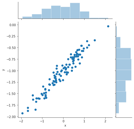
df = pd.DataFrame({"x" : x, "y" : y})

plt.close("all")
sp = sns.jointplot(x="x", y="y", data=df) # jointplot also gives the distributions of x and y in addition to the scatter plot
sns.despine()
sp.savefig("img/3.13.d_scatter.png", dpi=90)

3.13.d_scatter.png

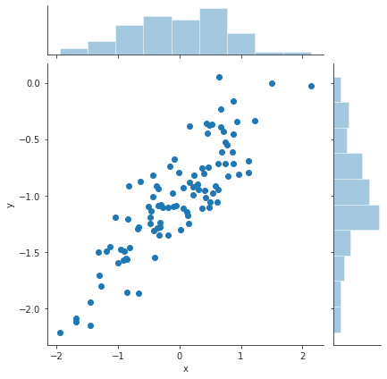
We can see a clear linear trend between x and y.

Least squares fit

model = smf.ols("y ~ x", data=df).fit()
print(model.summary())

                            OLS Regression Results
==============================================================================
Dep. Variable:                      y   R-squared:                       0.740
Model:                            OLS   Adj. R-squared:                  0.738
Method:                 Least Squares   F-statistic:                     279.2
Date:                Sat, 30 May 2020   Prob (F-statistic):           1.94e-30
Time:                        03:07:58   Log-Likelihood:               -0.24351
No. Observations:                 100   AIC:                             4.487
Df Residuals:                      98   BIC:                             9.697
Df Model:                           1
Covariance Type:            nonrobust
==============================================================================
                 coef    std err          t      P>|t|      [0.025      0.975]
------------------------------------------------------------------------------
Intercept     -1.0012      0.025    -40.774      0.000      -1.050      -0.952
x              0.5298      0.032     16.709      0.000       0.467       0.593
==============================================================================
Omnibus:                        2.996   Durbin-Watson:                   1.682
Prob(Omnibus):                  0.224   Jarque-Bera (JB):                2.971
Skew:                           0.409   Prob(JB):                        0.226
Kurtosis:                       2.787   Cond. No.                         1.30
==============================================================================

Warnings:
[1] Standard Errors assume that the covariance matrix of the errors is correctly specified.

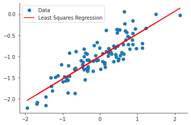
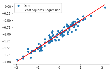
The estimates for $β_0$ and $β_1$ are almost equal to the true values. The true values fall within the 95% confidence interval of the estimated values.

ypred = model.predict(df["x"])

plt.close("all")
fig, ax = plt.subplots()
ax.plot(x, y, 'o', label="Data")
ax.plot(x, ypred, 'r', label="Least Squares Regression")
ax.legend(loc="best")
sns.despine()
fig.savefig("img/3.13.f_ols.png", dpi=90)

3.13.f_ols.png

Polynomial regression

poly_model = smf.ols(formula="y ~ x + I(x**2)", data=df).fit()
print(poly_model.summary())

                            OLS Regression Results
==============================================================================
Dep. Variable:                      y   R-squared:                       0.746
Model:                            OLS   Adj. R-squared:                  0.741
Method:                 Least Squares   F-statistic:                     142.6
Date:                Sat, 30 May 2020   Prob (F-statistic):           1.30e-29
Time:                        03:32:56   Log-Likelihood:                0.93852
No. Observations:                 100   AIC:                             4.123
Df Residuals:                      97   BIC:                             11.94
Df Model:                           2
Covariance Type:            nonrobust
==============================================================================
                 coef    std err          t      P>|t|      [0.025      0.975]
------------------------------------------------------------------------------
Intercept     -0.9732      0.031    -31.881      0.000      -1.034      -0.913
x              0.5200      0.032     16.177      0.000       0.456       0.584
I(x ** 2)     -0.0474      0.031     -1.523      0.131      -0.109       0.014
==============================================================================
Omnibus:                        2.591   Durbin-Watson:                   1.731
Prob(Omnibus):                  0.274   Jarque-Bera (JB):                2.542
Skew:                           0.380   Prob(JB):                        0.281
Kurtosis:                       2.818   Cond. No.                         2.08
==============================================================================

Warnings:
[1] Standard Errors assume that the covariance matrix of the errors is correctly specified.

The $R^2$ values of both the models are pretty much the same. Additionally the p-value of the quadratic term is not zero. The quadratic term does not improve the model fit.

Least squares fit with less noise

The new data is as follows. The spread of the noise is now 0.1 instead of 0.25.

eps = rng.normal(loc=0, scale=0.1, size=100)
y = -1 + 0.5 * x + eps

df2 = pd.DataFrame({"x" : x, "y" : y})

plt.close("all")
sp = sns.jointplot(x="x", y="y", data=df2) # jointplot also gives the distributions of x and y in addition to the scatter plot
sns.despine()
sp.savefig("img/3.13.h_scatter.png", dpi=90)

3.13.h_less_noisy_data.png

Now the least squares fit to this data.

less_noisy_model = smf.ols("y ~ x", data=df2).fit()
print(less_noisy_model.summary())

                            OLS Regression Results
==============================================================================
Dep. Variable:                      y   R-squared:                       0.935
Model:                            OLS   Adj. R-squared:                  0.934
Method:                 Least Squares   F-statistic:                     1403.
Date:                Sat, 30 May 2020   Prob (F-statistic):           7.01e-60
Time:                        03:39:50   Log-Likelihood:                 86.452
No. Observations:                 100   AIC:                            -168.9
Df Residuals:                      98   BIC:                            -163.7
Df Model:                           1
Covariance Type:            nonrobust
==============================================================================
                 coef    std err          t      P>|t|      [0.025      0.975]
------------------------------------------------------------------------------
Intercept     -1.0063      0.010    -97.523      0.000      -1.027      -0.986
x              0.4991      0.013     37.458      0.000       0.473       0.526
==============================================================================
Omnibus:                        3.211   Durbin-Watson:                   1.893
Prob(Omnibus):                  0.201   Jarque-Bera (JB):                2.554
Skew:                           0.345   Prob(JB):                        0.279
Kurtosis:                       3.371   Cond. No.                         1.30
==============================================================================

Warnings:
[1] Standard Errors assume that the covariance matrix of the errors is correctly specified.

The $R^2$ value for this data set is much larger than the original data set. The model is able to explain 93% of the less noisy data, whereas it could only explain around 70% of the original data set.

ypred = less_noisy_model.predict(df2["x"])

plt.close("all")
fig, ax = plt.subplots()
ax.plot(x, y, 'o', label="Data")
ax.plot(x, ypred, 'r', label="Least Squares Regression")
ax.legend(loc="best")
sns.despine()
fig.savefig("img/3.13.h_ols.png", dpi=90)

3.13.h_ols.png

Least squares fit with more noise

The new data is as follows. The spread of the noise is now 0.5 instead of 0.25.

eps = rng.normal(loc=0, scale=0.5, size=100)
y = -1 + 0.5 * x + eps

df3 = pd.DataFrame({"x" : x, "y" : y})

plt.close("all")
sp = sns.jointplot(x="x", y="y", data=df3)
sns.despine()
sp.savefig("img/3.13.i_scatter.png", dpi=90)

3.13.i_more_noisy_data.png

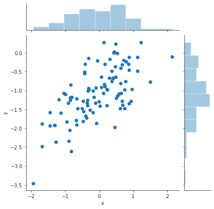
Now the least squares fit to this data.

more_noisy_model = smf.ols("y ~ x", data=df3).fit()
print(more_noisy_model.summary())

                            OLS Regression Results
==============================================================================
Dep. Variable:                      y   R-squared:                       0.430
Model:                            OLS   Adj. R-squared:                  0.424
Method:                 Least Squares   F-statistic:                     74.01
Date:                Sat, 30 May 2020   Prob (F-statistic):           1.29e-13
Time:                        03:45:50   Log-Likelihood:                -75.586
No. Observations:                 100   AIC:                             155.2
Df Residuals:                      98   BIC:                             160.4
Df Model:                           1
Covariance Type:            nonrobust
==============================================================================
                 coef    std err          t      P>|t|      [0.025      0.975]
------------------------------------------------------------------------------
Intercept     -1.0417      0.052    -19.971      0.000      -1.145      -0.938
x              0.5794      0.067      8.603      0.000       0.446       0.713
==============================================================================
Omnibus:                        0.119   Durbin-Watson:                   1.889
Prob(Omnibus):                  0.942   Jarque-Bera (JB):                0.294
Skew:                          -0.029   Prob(JB):                        0.863
Kurtosis:                       2.741   Cond. No.                         1.30
==============================================================================

Warnings:
[1] Standard Errors assume that the covariance matrix of the errors is correctly specified.

The $R^2$ value for this data set is much smaller than it was for the original data set. The model is able to explain only 43% of the more noisy data, whereas it could explain around 70% of the original data.

ypred = more_noisy_model.predict(df3["x"])

plt.close("all")
fig, ax = plt.subplots()
ax.plot(x, y, 'o', label="Data")
ax.plot(x, ypred, 'r', label="Least Squares Regression")
ax.legend(loc="best")
sns.despine()
fig.savefig("img/3.13.i_ols.png", dpi=90)

3.13.i_ols.png

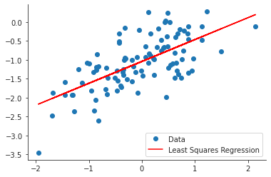
From the graph it appears that there are possible outliers, which is not surprising given the spread of the error.

Confidence intervals of the three models

print("Confidence interval based on original data set:\n")
print(f"{model.conf_int()}\n")
print("Confidence interval based on less noisy data set:\n")
print(f"{less_noisy_model.conf_int()}\n")
print("Confidence interval based on more noisy data set:\n")
print(f"{more_noisy_model.conf_int()}\n")

Confidence interval based on original data set:

                  0         1
Intercept -1.049887 -0.952433
x          0.466873  0.592714

Confidence interval based on less noisy data set:

                  0         1
Intercept -1.026756 -0.985803
x          0.472653  0.525535

Confidence interval based on more noisy data set:

                  0         1
Intercept -1.145197 -0.938180
x          0.445752  0.713071

The confidence intervals for the less noisy data set are the tightest and the confidence intervals for the more noisy data set are the loosest.

Question 14

Multiple linear model with collinearity

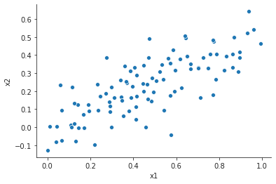
from numpy.random import MT19937

rng = np.random.default_rng(MT19937(seed=5))
x1 = rng.uniform(size=100)
x2 = 0.5 * x1 + rng.normal(size=100) / 10
y = 2 + 2 * x1 + 0.3 * x2 + rng.normal(size=100)

df_coll = pd.DataFrame({"x1" : x1, "x2" : x2, "y" : y})

The form of the linear model is

\begin{align} Y = 2 + 2 X_1 + 0.3 X_2 + ϵ. \end{align}

Correlation scatter plot

corr = df_coll.corr()
print(corr)

         x1       x2        y
x1  1.00000  0.76818  0.55569
x2  0.76818  1.00000  0.45415
y   0.55569  0.45415  1.00000

The correlation between x1 and x2 is 0.768.

plt.close("all")
fig, ax = plt.subplots()
sp = sns.scatterplot(x="x1", y="x2", data=df_coll, ax=ax)
sns.despine()
fig.savefig("img/3.14.a_scatter.png", dpi=90)

3.14.a_scatter.png

Least squares fit with `x1` and `x2`

coll_model1 = smf.ols("y ~ x1 + x2", data=df_coll).fit()
print(coll_model1.summary())

                            OLS Regression Results
==============================================================================
Dep. Variable:                      y   R-squared:                       0.311
Model:                            OLS   Adj. R-squared:                  0.296
Method:                 Least Squares   F-statistic:                     21.85
Date:                Sat, 30 May 2020   Prob (F-statistic):           1.46e-08
Time:                        04:51:30   Log-Likelihood:                -133.37
No. Observations:                 100   AIC:                             272.7
Df Residuals:                      97   BIC:                             280.6
Df Model:                           2
Covariance Type:            nonrobust
==============================================================================
                 coef    std err          t      P>|t|      [0.025      0.975]
------------------------------------------------------------------------------
Intercept      1.8690      0.194      9.651      0.000       1.485       2.253
x1             2.1749      0.568      3.832      0.000       1.048       3.301
x2             0.4454      0.881      0.505      0.614      -1.304       2.194
==============================================================================
Omnibus:                        0.484   Durbin-Watson:                   1.964
Prob(Omnibus):                  0.785   Jarque-Bera (JB):                0.623
Skew:                          -0.140   Prob(JB):                        0.732
Kurtosis:                       2.734   Cond. No.                         12.2
==============================================================================

Warnings:
[1] Standard Errors assume that the covariance matrix of the errors is correctly specified.

The estimated values for the coefficients are 1.869, 2.175, and 0.445 which are close to the true values, albeit with large standard errors, particularly for $\hat{β}_2$. Based on the p-values we can reject the null hypothesis for $β_1$, but we cannot reject the null-hypothesis for $β_2$.

Least squares fit with `x1` only

coll_model2 = smf.ols("y ~ x1", data=df_coll).fit()
print(coll_model2.summary())

                            OLS Regression Results
==============================================================================
Dep. Variable:                      y   R-squared:                       0.309
Model:                            OLS   Adj. R-squared:                  0.302
Method:                 Least Squares   F-statistic:                     43.78
Date:                Sat, 30 May 2020   Prob (F-statistic):           1.96e-09
Time:                        04:51:44   Log-Likelihood:                -133.50
No. Observations:                 100   AIC:                             271.0
Df Residuals:                      98   BIC:                             276.2
Df Model:                           1
Covariance Type:            nonrobust
==============================================================================
                 coef    std err          t      P>|t|      [0.025      0.975]
------------------------------------------------------------------------------
Intercept      1.8690      0.193      9.688      0.000       1.486       2.252
x1             2.3952      0.362      6.617      0.000       1.677       3.114
==============================================================================
Omnibus:                        0.538   Durbin-Watson:                   1.940
Prob(Omnibus):                  0.764   Jarque-Bera (JB):                0.650
Skew:                          -0.160   Prob(JB):                        0.723
Kurtosis:                       2.768   Cond. No.                         4.80
==============================================================================

Warnings:
[1] Standard Errors assume that the covariance matrix of the errors is correctly specified.

The coefficient value has increased, and the $R^2$ value has decreased marginally. We can still reject the null hypothesis based on the p-value.

Least squares fit with `x2` only

coll_model3 = smf.ols("y ~ x2", data=df_coll).fit()
print(coll_model3.summary())

                            OLS Regression Results
==============================================================================
Dep. Variable:                      y   R-squared:                       0.206
Model:                            OLS   Adj. R-squared:                  0.198
Method:                 Least Squares   F-statistic:                     25.46
Date:                Sat, 30 May 2020   Prob (F-statistic):           2.08e-06
Time:                        04:51:59   Log-Likelihood:                -140.42
No. Observations:                 100   AIC:                             284.8
Df Residuals:                      98   BIC:                             290.0
Df Model:                           1
Covariance Type:            nonrobust
==============================================================================
                 coef    std err          t      P>|t|      [0.025      0.975]
------------------------------------------------------------------------------
Intercept      2.2853      0.171     13.355      0.000       1.946       2.625
x2             3.0393      0.602      5.046      0.000       1.844       4.235
==============================================================================
Omnibus:                        0.036   Durbin-Watson:                   2.117
Prob(Omnibus):                  0.982   Jarque-Bera (JB):                0.064
Skew:                          -0.038   Prob(JB):                        0.969
Kurtosis:                       2.902   Cond. No.                         6.38
==============================================================================

Warnings:
[1] Standard Errors assume that the covariance matrix of the errors is correctly specified.

The coefficient value is much larger now, but the $R^2$ value has decreased. We can now reject the null hypothesis based on the p-value.

Contradiction of models

The three models do not contradict each other. Due to the high correlation between x1 and x2, we can predict x2 from x1. Thus in the original model x2 has very little explanatory power and so we cannot reject the null hypothesis for $β_2$.

For the second and third model the explanation for the increase in the coefficients is as follows. In the second model we are expressing x2 in terms of x1, and so the coefficient of x1 in the expression for y increases to 2.3. In the third model we are expressing x1 in terms of x2, and so the coefficient of x2 in the expression for y increases to 4.3. The 95% confidence interval of the second model includes the new true value of the coefficient. Even though the 95% confidence interval of the third model does not include the new true value of the coefficient it comes close. This is probably due to the difference between the random number generators used by R and numpy.

Additional data

df_coll = df_coll.append({"x1" : 0.1, "x2" : 0.8, "y" : 6}, ignore_index=True)

coll_model1 = smf.ols("y ~ x1 + x2", data=df_coll).fit()
coll_model2 = smf.ols("y ~ x1", data=df_coll).fit()
coll_model3 = smf.ols("y ~ x2", data=df_coll).fit()

print(coll_model1.summary())

                            OLS Regression Results
==============================================================================
Dep. Variable:                      y   R-squared:                       0.295
Model:                            OLS   Adj. R-squared:                  0.281
Method:                 Least Squares   F-statistic:                     20.50
Date:                Sat, 30 May 2020   Prob (F-statistic):           3.66e-08
Time:                        04:56:57   Log-Likelihood:                -138.91
No. Observations:                 101   AIC:                             283.8
Df Residuals:                      98   BIC:                             291.7
Df Model:                           2
Covariance Type:            nonrobust
==============================================================================
                 coef    std err          t      P>|t|      [0.025      0.975]
------------------------------------------------------------------------------
Intercept      1.9525      0.200      9.769      0.000       1.556       2.349
x1             1.2762      0.508      2.514      0.014       0.269       2.283
x2             2.0004      0.753      2.657      0.009       0.506       3.495
==============================================================================
Omnibus:                        0.020   Durbin-Watson:                   2.024
Prob(Omnibus):                  0.990   Jarque-Bera (JB):                0.144
Skew:                           0.018   Prob(JB):                        0.931
Kurtosis:                       2.819   Cond. No.                         9.92
==============================================================================

Warnings:
[1] Standard Errors assume that the covariance matrix of the errors is correctly specified.

print(coll_model2.summary())

                            OLS Regression Results
==============================================================================
Dep. Variable:                      y   R-squared:                       0.244
Model:                            OLS   Adj. R-squared:                  0.237
Method:                 Least Squares   F-statistic:                     31.98
Date:                Sat, 30 May 2020   Prob (F-statistic):           1.51e-07
Time:                        04:57:04   Log-Likelihood:                -142.43
No. Observations:                 101   AIC:                             288.9
Df Residuals:                      99   BIC:                             294.1
Df Model:                           1
Covariance Type:            nonrobust
==============================================================================
                 coef    std err          t      P>|t|      [0.025      0.975]
------------------------------------------------------------------------------
Intercept      2.0051      0.205      9.786      0.000       1.599       2.412
x1             2.1847      0.386      5.655      0.000       1.418       2.951
==============================================================================
Omnibus:                        6.115   Durbin-Watson:                   1.839
Prob(Omnibus):                  0.047   Jarque-Bera (JB):                7.252
Skew:                           0.308   Prob(JB):                       0.0266
Kurtosis:                       4.160   Cond. No.                         4.76
==============================================================================

Warnings:
[1] Standard Errors assume that the covariance matrix of the errors is correctly specified.

print(coll_model3.summary())

                            OLS Regression Results
==============================================================================
Dep. Variable:                      y   R-squared:                       0.249
Model:                            OLS   Adj. R-squared:                  0.242
Method:                 Least Squares   F-statistic:                     32.90
Date:                Sat, 30 May 2020   Prob (F-statistic):           1.06e-07
Time:                        04:57:12   Log-Likelihood:                -142.07
No. Observations:                 101   AIC:                             288.1
Df Residuals:                      99   BIC:                             293.4
Df Model:                           1
Covariance Type:            nonrobust
==============================================================================
                 coef    std err          t      P>|t|      [0.025      0.975]
------------------------------------------------------------------------------
Intercept      2.2419      0.168     13.365      0.000       1.909       2.575
x2             3.2762      0.571      5.736      0.000       2.143       4.409
==============================================================================
Omnibus:                        0.044   Durbin-Watson:                   2.139
Prob(Omnibus):                  0.978   Jarque-Bera (JB):                0.040
Skew:                          -0.033   Prob(JB):                        0.980
Kurtosis:                       2.927   Cond. No.                         6.09
==============================================================================

Warnings:
[1] Standard Errors assume that the covariance matrix of the errors is correctly specified.

The $R^2$ values for models 1 and 2 decreased. This observation decreased the predictive power of the models. The average leverage for the data set is

p = len(df_coll.columns)
n = len(df_coll)
lev = (p + 1) / n
print(f"{lev:.3f}")

0.040

plt.close("all")
fig, ax = plt.subplots()
rlplot = sm.graphics.influence_plot(coll_model1, criterion="Cooks", ax=ax)
sns.despine()
ax.set_xlabel("Leverage")
ax.set_ylabel("Standardized Residuals")
ax.set_title(" ")
fig.savefig("img/3.14.g_coll1_res_vs_lev.png", dpi=90)

3.14.g_coll1_res_vs_lev.png

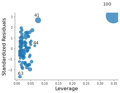
For the first model it is both an outlier and a high leverage point.

plt.close("all")
fig, ax = plt.subplots()
rlplot = sm.graphics.influence_plot(coll_model2, criterion="Cooks", ax=ax)
sns.despine()
ax.set_xlabel("Leverage")
ax.set_ylabel("Standardized Residuals")
ax.set_title(" ")
fig.savefig("img/3.14.g_coll2_res_vs_lev.png", dpi=90)

3.14.g_coll12_res_vs_lev.png

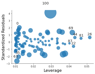
For the second model it is just an outlier.

plt.close("all")
fig, ax = plt.subplots()
rlplot = sm.graphics.influence_plot(coll_model3, criterion="Cooks", ax=ax)
sns.despine()
ax.set_xlabel("Leverage")
ax.set_ylabel("Standardized Residuals")
ax.set_title(" ")
fig.savefig("img/3.14.g_coll3_res_vs_lev.png", dpi=90)

3.14.g_coll3_res_vs_lev.png

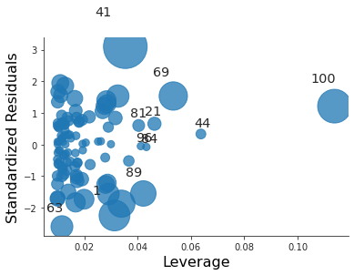
For the third model it is just an high leverage point.

Question 15

Predict per capita crime rate with the `Boston` data set

We load the Boston from statsmodels.

import statsmodels.api as sm

boston = sm.datasets.get_rdataset("Boston", "MASS")
print(boston.__doc__)

+--------+-----------------+
| Boston | R Documentation |
+--------+-----------------+

Housing Values in Suburbs of Boston
-----------------------------------

Description
~~~~~~~~~~~

The ``Boston`` data frame has 506 rows and 14 columns.

Usage
~~~~~

::

   Boston

Format
~~~~~~

This data frame contains the following columns:

``crim``
   per capita crime rate by town.

``zn``
   proportion of residential land zoned for lots over 25,000 sq.ft.

``indus``
   proportion of non-retail business acres per town.

``chas``
   Charles River dummy variable (= 1 if tract bounds river; 0
   otherwise).

``nox``
   nitrogen oxides concentration (parts per 10 million).

``rm``
   average number of rooms per dwelling.

``age``
   proportion of owner-occupied units built prior to 1940.

``dis``
   weighted mean of distances to five Boston employment centres.

``rad``
   index of accessibility to radial highways.

``tax``
   full-value property-tax rate per \\$10,000.

``ptratio``
   pupil-teacher ratio by town.

``black``
   *1000(Bk - 0.63)^2* where *Bk* is the proportion of blacks by town.

``lstat``
   lower status of the population (percent).

``medv``
   median value of owner-occupied homes in \\$1000s.

Source
~~~~~~

Harrison, D. and Rubinfeld, D.L. (1978) Hedonic prices and the demand
for clean air. *J. Environ. Economics and Management* **5**, 81–102.

Belsley D.A., Kuh, E. and Welsch, R.E. (1980) *Regression Diagnostics.
Identifying Influential Data and Sources of Collinearity.* New York:
Wiley.

Earlier we are fitted medv to the other predictors, now we will be fitting crim to the other predictors.

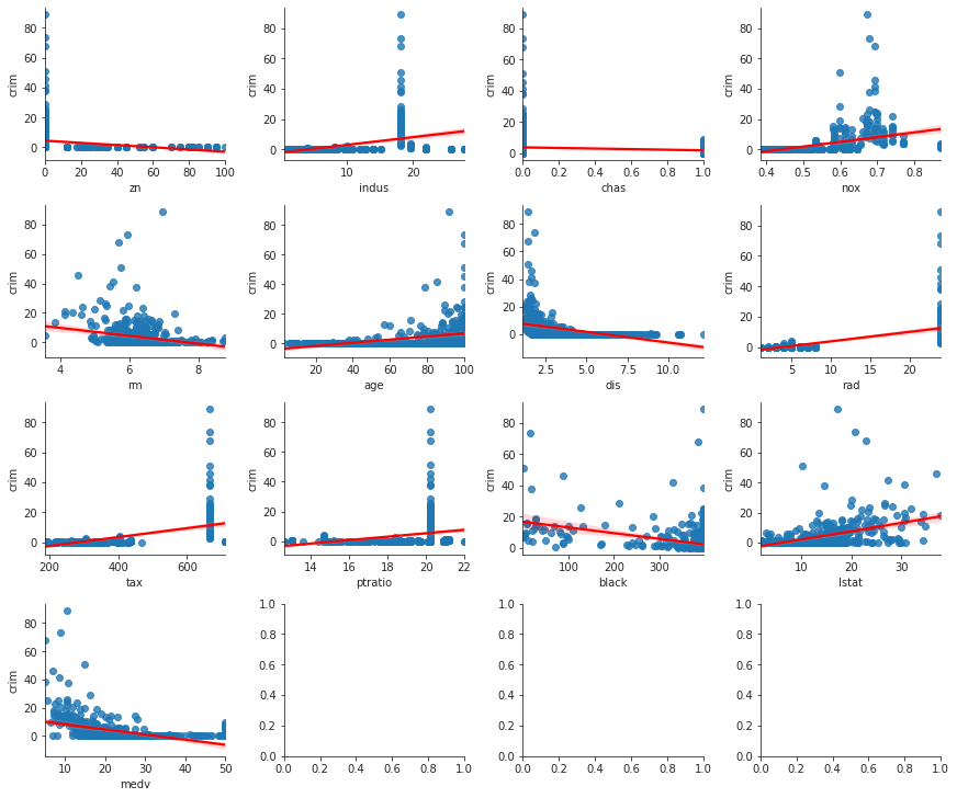
import statsmodels.formula.api as smf

df = boston.data
predictors = [c for c in df.columns if c != "crim"]
simple_models = {p : smf.ols(formula=f"crim ~ {p}", data=df).fit() for p in predictors}
print(f"predictor coefficient p-value")
for p, model in simple_models.items():
    print(f"{p:^9} {model.params[p]:>9,.4f} {model.pvalues[p]:>9,.4f}")

predictor coefficient p-value
   zn       -0.0739    0.0000
  indus      0.5098    0.0000
  chas      -1.8928    0.2094
   nox      31.2485    0.0000
   rm       -2.6841    0.0000
   age       0.1078    0.0000
   dis      -1.5509    0.0000
   rad       0.6179    0.0000
   tax       0.0297    0.0000
 ptratio     1.1520    0.0000
  black     -0.0363    0.0000
  lstat      0.5488    0.0000
  medv      -0.3632    0.0000

Except for chas everything else appears to be statistically significant.

import matplotlib.pyplot as plt
import seaborn as sns
from math import ceil

sns.set_style("ticks")
ncols = 4
nrows = ceil(len(predictors) / ncols)

plt.close("all")
fig, axs = plt.subplots(nrows=nrows, ncols=ncols, constrained_layout=True, figsize=(12, 10))
for i in range(nrows):
    for j in range(ncols):
        if i * ncols + j < len(predictors):
            sns.regplot(x=df[predictors[i * ncols + j]], y=df["crim"], ax=axs[i, j], line_kws={"color" : "r"})
            sns.despine()
fig.savefig("img/3.15.a_reg_mat.png", dpi=120)

3.15.a_reg_mat.png

Multiple regression with `Boston` data set

Y = df['crim']
X = df[predictors]
X = sm.add_constant(X)

ml_model = sm.OLS(Y, X).fit()
print(ml_model.summary())

                            OLS Regression Results
==============================================================================
Dep. Variable:                   crim   R-squared:                       0.454
Model:                            OLS   Adj. R-squared:                  0.440
Method:                 Least Squares   F-statistic:                     31.47
Date:                Sat, 30 May 2020   Prob (F-statistic):           1.57e-56
Time:                        12:26:02   Log-Likelihood:                -1653.3
No. Observations:                 506   AIC:                             3335.
Df Residuals:                     492   BIC:                             3394.
Df Model:                          13
Covariance Type:            nonrobust
==============================================================================
                 coef    std err          t      P>|t|      [0.025      0.975]
------------------------------------------------------------------------------
const         17.0332      7.235      2.354      0.019       2.818      31.248
zn             0.0449      0.019      2.394      0.017       0.008       0.082
indus         -0.0639      0.083     -0.766      0.444      -0.228       0.100
chas          -0.7491      1.180     -0.635      0.526      -3.068       1.570
nox          -10.3135      5.276     -1.955      0.051     -20.679       0.052
rm             0.4301      0.613      0.702      0.483      -0.774       1.634
age            0.0015      0.018      0.081      0.935      -0.034       0.037
dis           -0.9872      0.282     -3.503      0.001      -1.541      -0.433
rad            0.5882      0.088      6.680      0.000       0.415       0.761
tax           -0.0038      0.005     -0.733      0.464      -0.014       0.006
ptratio       -0.2711      0.186     -1.454      0.147      -0.637       0.095
black         -0.0075      0.004     -2.052      0.041      -0.015      -0.000
lstat          0.1262      0.076      1.667      0.096      -0.023       0.275
medv          -0.1989      0.061     -3.287      0.001      -0.318      -0.080
==============================================================================
Omnibus:                      666.613   Durbin-Watson:                   1.519
Prob(Omnibus):                  0.000   Jarque-Bera (JB):            84887.625
Skew:                           6.617   Prob(JB):                         0.00
Kurtosis:                      65.058   Cond. No.                     1.58e+04
==============================================================================

Warnings:
[1] Standard Errors assume that the covariance matrix of the errors is correctly specified.
[2] The condition number is large, 1.58e+04. This might indicate that there are
strong multicollinearity or other numerical problems.

Based on the p-values we can reject the null hypothesis for dis, rad, and medv. If we are willing to be less accurate we can also reject the null hypothesis for zn, nox, black, and lstat.

Comparison plot

import pandas as pd

ml_coefs = ml_model.params
sl_coefs = pd.Series({p : simple_models[p].params.loc[p] for p in predictors})
coef_df = pd.concat([sl_coefs, ml_coefs], axis=1)
coef_df.reset_index(inplace=True)
coef_df.columns = ["Predictors", "Simple OLS Coefficient", "Multiple OLS Coefficient"]
coef_df.dropna(inplace=True)
print(coef_df)

   Predictors  Simple OLS Coefficient  Multiple OLS Coefficient
0          zn               -0.073935                  0.044855
1       indus                0.509776                 -0.063855
2        chas               -1.892777                 -0.749134
3         nox               31.248531                -10.313535
4          rm               -2.684051                  0.430131
5         age                0.107786                  0.001452
6         dis               -1.550902                 -0.987176
7         rad                0.617911                  0.588209
8         tax                0.029742                 -0.003780
9     ptratio                1.151983                 -0.271081
10      black               -0.036280                 -0.007538
11      lstat                0.548805                  0.126211
12       medv               -0.363160                 -0.198887

plt.close("all")
fig, ax = plt.subplots()
sns.scatterplot(x="Simple OLS Coefficient", y="Multiple OLS Coefficient", data=coef_df, ax=ax)
sns.despine()
fig.savefig("img/3.15.c_comp_plot.png")

3.15.c_comp_plot.png

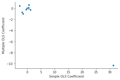
The coefficients for nox are very different in the two models.

Evidence of non-linear associations

We will use scikit-learn to generate the non-linear features.

from sklearn.preprocessing import PolynomialFeatures
pd.options.display.float_format = "{:,.3f}".format

Y = df['crim']
poly_features = PolynomialFeatures(degree=3)
poly_predictors = {p : poly_features.fit_transform(df[p][:, None]) for p in predictors}
poly_models = {p : sm.OLS(Y, poly_predictors[p]).fit() for p in predictors}
for p in predictors:
    print(f"p-values for {p}:")
    print(f"{poly_models[p].pvalues}\n")

p-values for zn:
const   0.000
x1      0.003
x2      0.094
x3      0.230
dtype: float64

p-values for indus:
const   0.020
x1      0.000
x2      0.000
x3      0.000
dtype: float64

p-values for chas:
const   0.000
x1      0.209
x2      0.209
x3      0.209
dtype: float64

p-values for nox:
const   0.000
x1      0.000
x2      0.000
x3      0.000
dtype: float64

p-values for rm:
const   0.081
x1      0.212
x2      0.364
x3      0.509
dtype: float64

p-values for age:
const   0.358
x1      0.143
x2      0.047
x3      0.007
dtype: float64

p-values for dis:
const   0.000
x1      0.000
x2      0.000
x3      0.000
dtype: float64

p-values for rad:
const   0.768
x1      0.623
x2      0.613
x3      0.482
dtype: float64

p-values for tax:
const   0.105
x1      0.110
x2      0.137
x3      0.244
dtype: float64

p-values for ptratio:
const   0.002
x1      0.003
x2      0.004
x3      0.006
dtype: float64

p-values for black:
const   0.000
x1      0.139
x2      0.474
x3      0.544
dtype: float64

p-values for lstat:
const   0.554
x1      0.335
x2      0.065
x3      0.130
dtype: float64

p-values for medv:
const   0.000
x1      0.000
x2      0.000
x3      0.000
dtype: float64

From the p-values we see that there is evidence of polynomial association between the response and the predictors indus, nox, age, dis, ptratio, and medv.

Linear Regression

Table of Contents

Notes

Accuracy

Outliers & High Leverage points

Exercises

Question 1

Question 2

Question 3

Question 4

Question 5

Question 6

Question 7

Question 8

Simple linear regression on Auto data set

Least squares plot

Diagnostic plots

Question 9

Scatter plot matrix of Auto data set

Correlation matrix

Multiple linear regression with Auto data set

Diagnostic plots

Interaction effects

Models with variable transformations

Question 10

Multiple regression with Carseats data set

Interpretation of coefficient of predictors

Linear model equation

Null hypothesis rejection

Smaller multiple linear model for Carseats sales

Confidence intervals of fitted parameters

Outliers and leverages

Question 11

Simple linear regression with synthetic data

Inverse simple linear relation with synthetic data

Relation between the two regressions

t-statistic for first model

t-statistic for second model

t-statistic for models with intercept

Question 12

Equal regression coefficients

Different coefficient estimates - numerical

Same coefficient estimates - numerical

Question 13

Feature vector

Error vector

Response vector

Scatter plot

Least squares fit

Polynomial regression

Least squares fit with less noise

Least squares fit with more noise

Confidence intervals of the three models

Question 14

Multiple linear model with collinearity

Correlation scatter plot

Least squares fit with x1 and x2

Least squares fit with x1 only

Least squares fit with x2 only

Contradiction of models

Additional data

Question 15

Predict per capita crime rate with the Boston data set

Multiple regression with Boston data set

Comparison plot

Evidence of non-linear associations

Simple linear regression on `Auto` data set

Scatter plot matrix of `Auto` data set

Multiple linear regression with `Auto` data set

Multiple regression with `Carseats` data set

Smaller multiple linear model for `Carseats` sales

Least squares fit with `x1` and `x2`

Least squares fit with `x1` only

Least squares fit with `x2` only

Predict per capita crime rate with the `Boston` data set

Multiple regression with `Boston` data set