Statistical Learning

Notes
Exercises

Notes

Inference is what statistics is mostly about, prediction is what machine learning is mostly about. – Statistics vs Machine Learning, fight!

Models

Parametric models reduce the problem of estimating \(f\) to estimating a few parameters. Easy to interpret, but might not fit the data well.
Non-parametric models do not assume any particular functional form for \(f\). Usually fit the data better than parametric models, given that there are large number of observations, much larger than that required by parametric models.

Learning

Supervised learning: For each observation \(i\) of predictor measurements \(x_i\) there is an associated response measurement \(y_i\).
Unsupervised learning: For each observation \(i\) there is a vector of measurements \(x_i\) but no associated response measurement.
Semi-supervised learning: Response measurements are available for some of the observations but not all.

Variables & Problems

Quantitative variables: numerical
Qualitative variables: categorical
Regression problems have quantitative response.
Classification problems have qualitative response.

Accuracy

There is no free lunch in statistics.

Mean squared error is typically used for regression problems.
Error rate, proportion of mistakes that are made if we apply the estimate \(\hat{f}\) to the data, is typically used for classification problems.
Test error rate is minimized by the Bayes Classifier.
Cross-validation is used to estimate test MSE using training data.
Variance is the change in the estimate \(\hat{f}\) of \(f\) due to change in training data.
Bias is the error due to approximating a complicated problem with a simpler model.
To reduce test error we need a model with low variance and low bias.
Increasing flexibility of the model generally decreases bias but increases variance.

Exercises

Question 1

(n > p) We can expect the performance of the flexible method to be better. With the large sample size, the flexible method will be able to better fit the data than the inflexible method.
(n < p) Since the sample size to small we can expect the flexible method to overfit. The inflexible method will perform better.
The inflexible method will suffer from high bias. The flexible method will perform better.
The flexible method might fit the erroneous observations. It will perform worse than the inflexible method.

Question 2

The response is quantitative. This is a regression problem. We are trying to infer how does the CEO salary depend on the various factors. We are not trying to predict the CEO salary.
The response is qualitative. This is a classification problem. We are trying to predict whether the product will be a success or a failure.
The response is qualitative. This is a regression problem. We are interested in prediction.

Question 3

The sketches are as follows:

import numpy as np
import matplotlib.pyplot as plt
import seaborn as sns

sns.set_style("ticks")

flexibility = np.linspace(0, 10, 100)
squared_bias = 0.02 * (10 - flexibility) ** 2
variance = 0.02 * flexibility ** 2
training_error = 0.003 * (10 - flexibility) ** 3
test_error = 3 - 0.6 * flexibility + 0.06 * flexibility ** 2
bayes_error = np.ones_like(flexibility)

plt.close('all') # To prevent memory consumption
fig, ax = plt.subplots()
ax.plot(flexibility, squared_bias, label="Bias")
ax.plot(flexibility, variance, label="Variance")
ax.plot(flexibility, training_error, label="Training Error")
ax.plot(flexibility, test_error, label="Test Error")
ax.plot(flexibility, bayes_error, label="Bayes Error")
ax.set_xlabel("Flexibility")
ax.legend(loc="upper center")

sns.despine()

fig.savefig("img/bv-decomp.png", dpi=90)

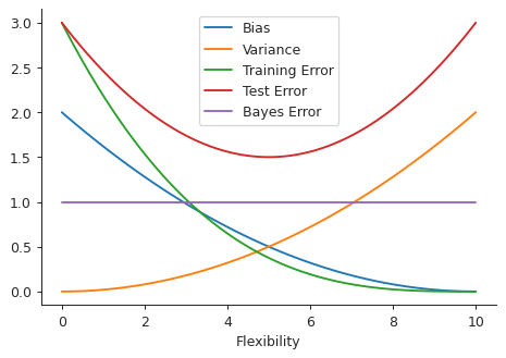
These graphs are not exact representations of how actual bias, variance, etc. would look, but an estimation that conveys the general idea.

The (squared) bias decreases with increasing flexibility because the model fits to the data better and better. On the other hand the model is more sensitive to training data with increasing flexibility, resulting in the increasing trend for the variance.

The training error is similar to the bias, for classification problems. The test error initially decreases since with increasing flexibility the model has a better chance of predicting the test response. However beyond a certain flexibility it is overfitted to the training data and gives sub-optimal results with the test data.

The Bayes error is independent of the flexibility of the model. It completely depends on the data.

Question 4

Three real-life applications of classification are:
- Predicting if an email is spam or non-spam.
- Predicting if a customer will remain loyal to the brand or not.
Three real-life applications of regression are:
- Predicting real estate prices based on certain factors, like location, size, etc. The price will be the response, and location, size, etc. will be the predictors.
Three real-life applications of cluster analysis are:
- Grouping galaxies based on the profile of the light that they emit.
- Checking how similar two documents are. This could be useful in preventing plagiarism.

Question 5

Advantages:

Flexible approach is better able to fit the training data.
Flexible approach might be able to estimate the underlying function better than the inflexible approach.

Disadvantages:

Flexible approaches are prone to overfitting.
Flexible approaches are more difficult to interpret than inflexible approaches.

A more flexible approach is more suitable when we are interested in prediction and a large amount of training data is available. A less flexible approach is more suitable when we are interested in inference, or if we do not have sufficient data.

Question 6

In a parametric approach we first choose a model to fit the data to. This reduces the problem of estimating the true function to estimating the models of the parameter. Non-parametric approaches do not make any assumption about the form of the true function. One advantage of a parametric approach is that it does not require as much training data as a non-parametric approach. It also easier to interpret and less prone to overfitting. On the other hand the model used in a parametric approach might be nothing like the true function.

Question 7

The data is as follows:

Obs.	X₁	X₂	X₃	Y
1	0	3	0	Red
2	2	0	0	Red
3	0	1	3	Red
4	0	1	2	Green
5	-1	0	1	Green
6	1	1	1	Red

The test point is X₁ = X₂ = X₃ = 0. The Euclidean distance between the observations and the test point are calculated as follows:

import pandas as pd
from tabulate import tabulate

df = pd.DataFrame.from_dict({'X1': [0, 2, 0, 0, -1, 1], 'X2': [3, 0, 1, 1, 0, 1], 'X3': [0, 0, 3, 2, 1, 1], 'Y':['Red', 'Red', 'Red', 'Green', 'Green', 'Red']})
test = np.array([0, 0, 0])
df['Distance'] = np.linalg.norm(df[['X1', 'X2', 'X3']].values-test, axis=1)
pd.set_option('precision', 5)
print(tabulate(df, df.columns, tablefmt="orgtbl"))

|    |   X1 |   X2 |   X3 | Y     |   Distance |
|----+------+------+------+-------+------------|
|  0 |    0 |    3 |    0 | Red   |    3       |
|  1 |    2 |    0 |    0 | Red   |    2       |
|  2 |    0 |    1 |    3 | Red   |    3.16228 |
|  3 |    0 |    1 |    2 | Green |    2.23607 |
|  4 |   -1 |    0 |    1 | Green |    1.41421 |
|  5 |    1 |    1 |    1 | Red   |    1.73205 |

If \(K = 1\), then the prediction is Green. From the above table we see that the test point is closest to the fifth observations, and so classify it in the same group as the fifth observation.

For \(K = 3\), the neighbors are observations 2, 5, and 6. The responses for 2 and 6 are Red. The response for 5 is Green. The probability for being Red is higher than being Green (2/3 > 1/3). Using the idea of the Bayes classifier we predict that the response will be Red.

If the Bayes decision boundary is highly nonlinear then the best value for \(K\) will be small. A smaller \(K\) results in more granular grouping, that is for small \(K\) the decision boundary is better able to capture the local non-linearities, because there will be very few neighbors.

Question 8

The `College` data set

college = pd.read_csv("data/College.csv")
print(tabulate(college.head(), college.columns, tablefmt="orgtbl"))

|    | Unnamed: 0                   | Private   |   Apps |   Accept |   Enroll |   Top10perc |   Top25perc |   F.Undergrad |   P.Undergrad |   Outstate |   Room.Board |   Books |   Personal |   PhD |   Terminal |   S.F.Ratio |   perc.alumni |   Expend |   Grad.Rate |
|----+------------------------------+-----------+--------+----------+----------+-------------+-------------+---------------+---------------+------------+--------------+---------+------------+-------+------------+-------------+---------------+----------+-------------|
|  0 | Abilene Christian University | Yes       |   1660 |     1232 |      721 |          23 |          52 |          2885 |           537 |       7440 |         3300 |     450 |       2200 |    70 |         78 |        18.1 |            12 |     7041 |          60 |
|  1 | Adelphi University           | Yes       |   2186 |     1924 |      512 |          16 |          29 |          2683 |          1227 |      12280 |         6450 |     750 |       1500 |    29 |         30 |        12.2 |            16 |    10527 |          56 |
|  2 | Adrian College               | Yes       |   1428 |     1097 |      336 |          22 |          50 |          1036 |            99 |      11250 |         3750 |     400 |       1165 |    53 |         66 |        12.9 |            30 |     8735 |          54 |
|  3 | Agnes Scott College          | Yes       |    417 |      349 |      137 |          60 |          89 |           510 |            63 |      12960 |         5450 |     450 |        875 |    92 |         97 |         7.7 |            37 |    19016 |          59 |
|  4 | Alaska Pacific University    | Yes       |    193 |      146 |       55 |          16 |          44 |           249 |           869 |       7560 |         4120 |     800 |       1500 |    76 |         72 |        11.9 |             2 |    10922 |          15 |

College names as index

college.set_index("Unnamed: 0", inplace=True)
college.index.name = "Names"

headers = [college.index.name] + list(college.columns)
print(tabulate(college.head(), headers, tablefmt="orgtbl"))

| Names                        | Private   |   Apps |   Accept |   Enroll |   Top10perc |   Top25perc |   F.Undergrad |   P.Undergrad |   Outstate |   Room.Board |   Books |   Personal |   PhD |   Terminal |   S.F.Ratio |   perc.alumni |   Expend |   Grad.Rate |
|------------------------------+-----------+--------+----------+----------+-------------+-------------+---------------+---------------+------------+--------------+---------+------------+-------+------------+-------------+---------------+----------+-------------|
| Abilene Christian University | Yes       |   1660 |     1232 |      721 |          23 |          52 |          2885 |           537 |       7440 |         3300 |     450 |       2200 |    70 |         78 |        18.1 |            12 |     7041 |          60 |
| Adelphi University           | Yes       |   2186 |     1924 |      512 |          16 |          29 |          2683 |          1227 |      12280 |         6450 |     750 |       1500 |    29 |         30 |        12.2 |            16 |    10527 |          56 |
| Adrian College               | Yes       |   1428 |     1097 |      336 |          22 |          50 |          1036 |            99 |      11250 |         3750 |     400 |       1165 |    53 |         66 |        12.9 |            30 |     8735 |          54 |
| Agnes Scott College          | Yes       |    417 |      349 |      137 |          60 |          89 |           510 |            63 |      12960 |         5450 |     450 |        875 |    92 |         97 |         7.7 |            37 |    19016 |          59 |
| Alaska Pacific University    | Yes       |    193 |      146 |       55 |          16 |          44 |           249 |           869 |       7560 |         4120 |     800 |       1500 |    76 |         72 |        11.9 |             2 |    10922 |          15 |

Summary of data

print(tabulate(college.describe(), college.columns, tablefmt="orgtbl"))

| Private   |     Apps |   Accept |   Enroll |   Top10perc |   Top25perc |   F.Undergrad |   P.Undergrad |   Outstate |   Room.Board |    Books |   Personal |      PhD |   Terminal |   S.F.Ratio |   perc.alumni |   Expend |   Grad.Rate |
|-----------+----------+----------+----------+-------------+-------------+---------------+---------------+------------+--------------+----------+------------+----------+------------+-------------+---------------+----------+-------------|
| count     |   777    |   777    |  777     |    777      |    777      |        777    |       777     |     777    |       777    |  777     |    777     | 777      |   777      |   777       |      777      |   777    |    777      |
| mean      |  3001.64 |  2018.8  |  779.973 |     27.5586 |     55.7967 |       3699.91 |       855.299 |   10440.7  |      4357.53 |  549.381 |   1340.64  |  72.6602 |    79.7027 |    14.0897  |       22.7439 |  9660.17 |     65.4633 |
| std       |  3870.2  |  2451.11 |  929.176 |     17.6404 |     19.8048 |       4850.42 |      1522.43  |    4023.02 |      1096.7  |  165.105 |    677.071 |  16.3282 |    14.7224 |     3.95835 |       12.3918 |  5221.77 |     17.1777 |
| min       |    81    |    72    |   35     |      1      |      9      |        139    |         1     |    2340    |      1780    |   96     |    250     |   8      |    24      |     2.5     |        0      |  3186    |     10      |
| 25%       |   776    |   604    |  242     |     15      |     41      |        992    |        95     |    7320    |      3597    |  470     |    850     |  62      |    71      |    11.5     |       13      |  6751    |     53      |
| 50%       |  1558    |  1110    |  434     |     23      |     54      |       1707    |       353     |    9990    |      4200    |  500     |   1200     |  75      |    82      |    13.6     |       21      |  8377    |     65      |
| 75%       |  3624    |  2424    |  902     |     35      |     69      |       4005    |       967     |   12925    |      5050    |  600     |   1700     |  85      |    92      |    16.5     |       31      | 10830    |     78      |
| max       | 48094    | 26330    | 6392     |     96      |    100      |      31643    |     21836     |   21700    |      8124    | 2340     |   6800     | 103      |   100      |    39.8     |       64      | 56233    |    118      |

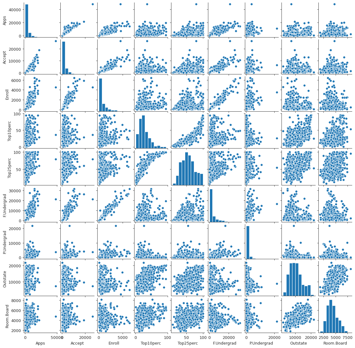
Scatter plot matrix

plot_columns = list(college.columns)[:10]
plt.close('all')
spm = sns.pairplot(college[plot_columns])
spm.fig.set_size_inches(12, 12)
spm.savefig("img/college_scatter.png", dpi=90)

Box plots

plt.close('all')
bp1 = sns.boxplot(x="Private", y="Outstate", data=college)
sns.despine()
plt.tight_layout()
bp1.get_figure().savefig("img/college_outstate_private.png", dpi=90)

Elite universities

college["Elite"] = college["Top10perc"].apply(lambda x: "Yes" if x > 50 else "No")
print(college["Elite"].value_counts())

No     699
Yes     78
Name: Elite, dtype: int64

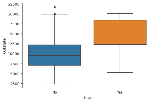
There are 78 elite universities, where more than 50% of their students come from the top 10% of their high school classes.

plt.close('all')
bp2 = sns.boxplot(x="Elite", y="Outstate", data=college)
sns.despine()
plt.tight_layout()
bp2.get_figure().savefig("img/college_outstate_elite.png", dpi=90)

Binning and histograms

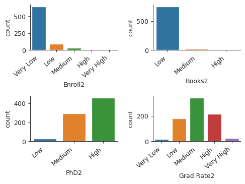
We are going to produce histograms for some of the quantitative variables with differing number of bins. We first need to bin these quantitative variables.

print(college.info())

<class 'pandas.core.frame.DataFrame'>
Index: 777 entries, Abilene Christian University to York College of Pennsylvania
Data columns (total 19 columns):
 #   Column       Non-Null Count  Dtype
---  ------       --------------  -----
 0   Private      777 non-null    object
 1   Apps         777 non-null    int64
 2   Accept       777 non-null    int64
 3   Enroll       777 non-null    int64
 4   Top10perc    777 non-null    int64
 5   Top25perc    777 non-null    int64
 6   F.Undergrad  777 non-null    int64
 7   P.Undergrad  777 non-null    int64
 8   Outstate     777 non-null    int64
 9   Room.Board   777 non-null    int64
 10  Books        777 non-null    int64
 11  Personal     777 non-null    int64
 12  PhD          777 non-null    int64
 13  Terminal     777 non-null    int64
 14  S.F.Ratio    777 non-null    float64
 15  perc.alumni  777 non-null    int64
 16  Expend       777 non-null    int64
 17  Grad.Rate    777 non-null    int64
 18  Elite        777 non-null    object
dtypes: float64(1), int64(16), object(2)
memory usage: 141.4+ KB
None

We see that there are 17 quantitative variables. For this activity I will choose Enroll, Books, PhD, and Grad.Rate as the quantitative variables to plot. To keep things simple we will bin these variables in to either 3 bins or 5 bins.

cut_bins3 = ["Low", "Medium", "High"]
cut_bins5 = ["Very Low", "Low", "Medium", "High", "Very High"]
college["Enroll2"] = pd.cut(college["Enroll"], 5, labels=cut_bins5)
college["Books2"] = pd.cut(college["Books"], 3, labels=cut_bins3)
college["PhD2"] = pd.cut(college["PhD"], 3, labels=cut_bins3)
college["Grad.Rate2"] = pd.cut(college["Grad.Rate"], 5, labels=cut_bins5)

plt.close("all")
fig, axs = plt.subplots(2, 2)
sns.countplot(college["Enroll2"], ax=axs[0, 0])
sns.countplot(college["Books2"], ax=axs[0, 1])
sns.countplot(college["PhD2"], ax=axs[1, 0])
sns.countplot(college["Grad.Rate2"], ax=axs[1, 1])
sns.despine()

axs[0, 0].set_xticklabels(axs[0, 0].get_xticklabels(), rotation=40, ha="right")
axs[0, 1].set_xticklabels(axs[0, 1].get_xticklabels(), rotation=40, ha="right")
axs[1, 0].set_xticklabels(axs[1, 0].get_xticklabels(), rotation=40, ha="right")
axs[1, 1].set_xticklabels(axs[1, 1].get_xticklabels(), rotation=40, ha="right")

plt.subplots_adjust(wspace=0.4, hspace=1)
fig.savefig("img/college_hist.png", dpi=90)

Question 9

Predictors of the `Auto` data set

auto = pd.read_csv("data/Auto.csv")
auto.dropna(inplace=True)
print(auto.info())

<class 'pandas.core.frame.DataFrame'>
Int64Index: 397 entries, 0 to 396
Data columns (total 9 columns):
 #   Column        Non-Null Count  Dtype
---  ------        --------------  -----
 0   mpg           397 non-null    float64
 1   cylinders     397 non-null    int64
 2   displacement  397 non-null    float64
 3   horsepower    397 non-null    object
 4   weight        397 non-null    int64
 5   acceleration  397 non-null    float64
 6   year          397 non-null    int64
 7   origin        397 non-null    int64
 8   name          397 non-null    object
dtypes: float64(3), int64(4), object(2)
memory usage: 31.0+ KB
None

We see that there are two qualitative predictors, horsepower and name. While name is expected to be qualitative, horsepower should presumably be quantitative. We should check the data in the horsepower column and see if we can convert that to a numeric form.

print(auto["horsepower"].unique())

['130' '165' '150' '140' '198' '220' '215' '225' '190' '170' '160' '95'
 '97' '85' '88' '46' '87' '90' '113' '200' '210' '193' '?' '100' '105'
 '175' '153' '180' '110' '72' '86' '70' '76' '65' '69' '60' '80' '54'
 '208' '155' '112' '92' '145' '137' '158' '167' '94' '107' '230' '49' '75'
 '91' '122' '67' '83' '78' '52' '61' '93' '148' '129' '96' '71' '98' '115'
 '53' '81' '79' '120' '152' '102' '108' '68' '58' '149' '89' '63' '48'
 '66' '139' '103' '125' '133' '138' '135' '142' '77' '62' '132' '84' '64'
 '74' '116' '82']

So the reason that horsepower is not numeric is because there are some missing values which are represented by "?". We need to remove the rows containing the missing data, and then make this column numeric.

auto.drop(auto[auto.horsepower == "?"].index, inplace=True)
auto["horsepower"] = pd.to_numeric(auto["horsepower"])
print(auto.info())

<class 'pandas.core.frame.DataFrame'>
Int64Index: 392 entries, 0 to 396
Data columns (total 9 columns):
 #   Column        Non-Null Count  Dtype
---  ------        --------------  -----
 0   mpg           392 non-null    float64
 1   cylinders     392 non-null    int64
 2   displacement  392 non-null    float64
 3   horsepower    392 non-null    int64
 4   weight        392 non-null    int64
 5   acceleration  392 non-null    float64
 6   year          392 non-null    int64
 7   origin        392 non-null    int64
 8   name          392 non-null    object
dtypes: float64(3), int64(5), object(1)
memory usage: 30.6+ KB
None

Now only name is the qualitative predictor.

Range of quantitative predictors

from pprint import pprint

quant = auto.select_dtypes(exclude="object").columns
ranges = {col: (min(auto[col]), max(auto[col])) for col in quant}
pprint(ranges)

{'acceleration': (8.0, 24.8),
 'cylinders': (3, 8),
 'displacement': (68.0, 455.0),
 'horsepower': (46, 230),
 'mpg': (9.0, 46.6),
 'origin': (1, 3),
 'weight': (1613, 5140),
 'year': (70, 82)}

Mean and standard deviation of quantitative predictors

msd = {col: {"mean": round(np.mean(auto[col]), 2), "std": round(np.std(auto[col]), 2)} for col in quant}
pprint(msd)

# An alternative is to use the following aggregrate method:
# auto.agg(["mean", "std"])

{'acceleration': {'mean': 15.54, 'std': 2.76},
 'cylinders': {'mean': 5.47, 'std': 1.7},
 'displacement': {'mean': 194.41, 'std': 104.51},
 'horsepower': {'mean': 104.47, 'std': 38.44},
 'mpg': {'mean': 23.45, 'std': 7.8},
 'origin': {'mean': 1.58, 'std': 0.8},
 'weight': {'mean': 2977.58, 'std': 848.32},
 'year': {'mean': 75.98, 'std': 3.68}}

Data subset

We remove the 10^th through 85^th observations, and then calculate the ranges, mean and standard deviation of the remaining data set.

auto2 = auto.drop(auto.index[10:85])

ranges = {col: (min(auto2[col]), max(auto2[col])) for col in quant}
pprint(ranges)

{'acceleration': (8.5, 24.8),
 'cylinders': (3, 8),
 'displacement': (68.0, 455.0),
 'horsepower': (46, 230),
 'mpg': (11.0, 46.6),
 'origin': (1, 3),
 'weight': (1649, 4997),
 'year': (70, 82)}

msd = {col: {"mean": round(np.mean(auto[col]), 2), "std": round(np.std(auto[col]), 2)} for col in quant}
pprint(msd)

{'acceleration': {'mean': 15.54, 'std': 2.76},
 'cylinders': {'mean': 5.47, 'std': 1.7},
 'displacement': {'mean': 194.41, 'std': 104.51},
 'horsepower': {'mean': 104.47, 'std': 38.44},
 'mpg': {'mean': 23.45, 'std': 7.8},
 'origin': {'mean': 1.58, 'std': 0.8},
 'weight': {'mean': 2977.58, 'std': 848.32},
 'year': {'mean': 75.98, 'std': 3.68}}

Pair plots

plt.close('all')
spm = sns.pairplot(auto[["mpg", "horsepower", "weight", "displacement", "acceleration"]])
spm.fig.set_size_inches(6, 6)
spm.savefig("img/auto_pair.png")

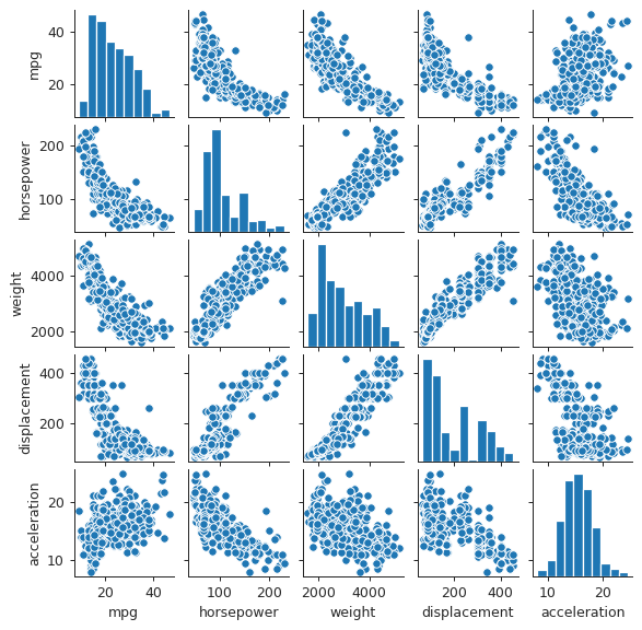
We observe that the gas mileage mpg decreases somewhat linearly as horsepower, weight, and displacement increases. This seems reasonable. Similarly displacement is positively correlated to weight and horsepower. The relation between acceleration and the other variables is not easy to interpret from these plots.

Predicting gas mileage

As we observed earlier that mpg has a linear relation with horsepower, weight, and displacement. We can therefore use that to predict mpg.

Question 10

Boston data set

from sklearn.datasets import load_boston

lb = load_boston()
boston = pd.DataFrame(lb.data, columns=lb.feature_names)
boston['MEDV'] = lb.target
print(tabulate(boston.head(), boston.columns, tablefmt="orgtbl"))

|    |    CRIM |   ZN |   INDUS |   CHAS |   NOX |    RM |   AGE |    DIS |   RAD |   TAX |   PTRATIO |      B |   LSTAT |   MEDV |
|----+---------+------+---------+--------+-------+-------+-------+--------+-------+-------+-----------+--------+---------+--------|
|  0 | 0.00632 |   18 |    2.31 |      0 | 0.538 | 6.575 |  65.2 | 4.09   |     1 |   296 |      15.3 | 396.9  |    4.98 |   24   |
|  1 | 0.02731 |    0 |    7.07 |      0 | 0.469 | 6.421 |  78.9 | 4.9671 |     2 |   242 |      17.8 | 396.9  |    9.14 |   21.6 |
|  2 | 0.02729 |    0 |    7.07 |      0 | 0.469 | 7.185 |  61.1 | 4.9671 |     2 |   242 |      17.8 | 392.83 |    4.03 |   34.7 |
|  3 | 0.03237 |    0 |    2.18 |      0 | 0.458 | 6.998 |  45.8 | 6.0622 |     3 |   222 |      18.7 | 394.63 |    2.94 |   33.4 |
|  4 | 0.06905 |    0 |    2.18 |      0 | 0.458 | 7.147 |  54.2 | 6.0622 |     3 |   222 |      18.7 | 396.9  |    5.33 |   36.2 |

print(lb['DESCR'])

.. _boston_dataset:

Boston house prices dataset
---------------------------

**Data Set Characteristics:**

    :Number of Instances: 506

    :Number of Attributes: 13 numeric/categorical predictive. Median Value (attribute 14) is usually the target.

    :Attribute Information (in order):
        - CRIM     per capita crime rate by town
        - ZN       proportion of residential land zoned for lots over 25,000 sq.ft.
        - INDUS    proportion of non-retail business acres per town
        - CHAS     Charles River dummy variable (= 1 if tract bounds river; 0 otherwise)
        - NOX      nitric oxides concentration (parts per 10 million)
        - RM       average number of rooms per dwelling
        - AGE      proportion of owner-occupied units built prior to 1940
        - DIS      weighted distances to five Boston employment centres
        - RAD      index of accessibility to radial highways
        - TAX      full-value property-tax rate per $10,000
        - PTRATIO  pupil-teacher ratio by town
        - B        1000(Bk - 0.63)^2 where Bk is the proportion of blacks by town
        - LSTAT    % lower status of the population
        - MEDV     Median value of owner-occupied homes in $1000's

    :Missing Attribute Values: None

    :Creator: Harrison, D. and Rubinfeld, D.L.

This is a copy of UCI ML housing dataset.
https://archive.ics.uci.edu/ml/machine-learning-databases/housing/


This dataset was taken from the StatLib library which is maintained at Carnegie Mellon University.

The Boston house-price data of Harrison, D. and Rubinfeld, D.L. 'Hedonic
prices and the demand for clean air', J. Environ. Economics & Management,
vol.5, 81-102, 1978.   Used in Belsley, Kuh & Welsch, 'Regression diagnostics
...', Wiley, 1980.   N.B. Various transformations are used in the table on
pages 244-261 of the latter.

The Boston house-price data has been used in many machine learning papers that address regression
problems.

.. topic:: References

   - Belsley, Kuh & Welsch, 'Regression diagnostics: Identifying Influential Data and Sources of Collinearity', Wiley, 1980. 244-261.
   - Quinlan,R. (1993). Combining Instance-Based and Model-Based Learning. In Proceedings on the Tenth International Conference of Machine Learning, 236-243, University of Massachusetts, Amherst. Morgan Kaufmann.

There are 506 rows, and 14 columns in this data set. The last column shows the median value of owner-occupied homes in Boston suburbs, and the other columns show the values of the different factors / predictors, on which the median value presumably depends. The rows show the data collected for 506 houses in Boston suburbs.

Pair plots

plt.close("all")
spm = sns.pairplot(boston, plot_kws = {'s': 10})
spm.fig.set_size_inches(12, 12)
spm.savefig("img/boston_scatter.png", dpi=90)

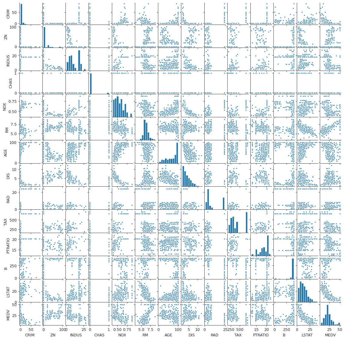
Looking at the plots we can easily identify that the median value has a positive linear correlation with the number of rooms (RM), and a negative, possibly non-linear, correlation with the "% lower status of the population" (LSTAT). We also see that RM has a negative correlation with LSTAT. This makes sense, since houses with more rooms are expected to be more expensive, and someone belonging to the low-income group will not be able to afford such a house. It is harder to determine from the plot how does the median value depend on the other predictors.

Association with per capita crime rate

print(boston.corrwith(boston["CRIM"]).sort_values())

MEDV      -0.388305
B         -0.385064
DIS       -0.379670
RM        -0.219247
ZN        -0.200469
CHAS      -0.055892
PTRATIO    0.289946
AGE        0.352734
INDUS      0.406583
NOX        0.420972
LSTAT      0.455621
TAX        0.582764
RAD        0.625505
CRIM       1.000000
dtype: float64

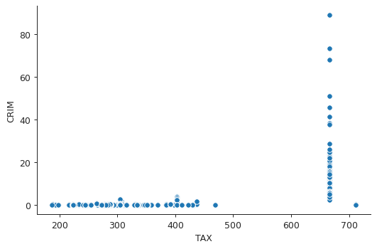
From the correlation values we can expect RAD (accessibility to radial highways) and TAX (property tax rates) to be associated with the per capita crime rate.

plt.close("all")
sns.scatterplot(x="TAX", y="CRIM", data=boston)
sns.despine()
plt.tight_layout()
plt.savefig("img/boston_crim_tax.png", dpi=90)

plt.close("all")
sns.boxplot(x="RAD", y="CRIM", data=boston)
sns.despine()
plt.tight_layout()
plt.savefig("img/boston_crim_rad.png", dpi=90)

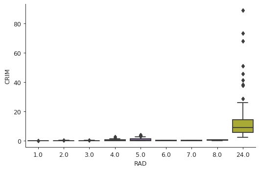
These plots show that the average per capita crime rate is much higher when the tax rate is \(~ 660\) or the index of accessibility to radial highways is 24.

Predictor ranges

ranges = {col: (boston[col].min(), boston[col].max()) for col in boston.columns[:-1]}
pprint(ranges)

{'AGE': (2.9, 100.0),
 'B': (0.32, 396.9),
 'CHAS': (0.0, 1.0),
 'CRIM': (0.00632, 88.9762),
 'DIS': (1.1296, 12.1265),
 'INDUS': (0.46, 27.74),
 'LSTAT': (1.73, 37.97),
 'NOX': (0.385, 0.871),
 'PTRATIO': (12.6, 22.0),
 'RAD': (1.0, 24.0),
 'RM': (3.561, 8.78),
 'TAX': (187.0, 711.0),
 'ZN': (0.0, 100.0)}

The per capita crime rate varies a lot across Boston suburbs, from a low of 0.00632 to a high of 88.9762. This shows that there are suburbs that have particularly high crime rates:

high_crime = boston.nlargest(5, "CRIM")
print(tabulate(high_crime, boston.columns, tablefmt="orgtbl"))

|     |    CRIM |   ZN |   INDUS |   CHAS |   NOX |    RM |   AGE |    DIS |   RAD |   TAX |   PTRATIO |      B |   LSTAT |   MEDV |
|-----+---------+------+---------+--------+-------+-------+-------+--------+-------+-------+-----------+--------+---------+--------|
| 380 | 88.9762 |    0 |    18.1 |      0 | 0.671 | 6.968 |  91.9 | 1.4165 |    24 |   666 |      20.2 | 396.9  |   17.21 |   10.4 |
| 418 | 73.5341 |    0 |    18.1 |      0 | 0.679 | 5.957 | 100   | 1.8026 |    24 |   666 |      20.2 |  16.45 |   20.62 |    8.8 |
| 405 | 67.9208 |    0 |    18.1 |      0 | 0.693 | 5.683 | 100   | 1.4254 |    24 |   666 |      20.2 | 384.97 |   22.98 |    5   |
| 410 | 51.1358 |    0 |    18.1 |      0 | 0.597 | 5.757 | 100   | 1.413  |    24 |   666 |      20.2 |   2.6  |   10.11 |   15   |
| 414 | 45.7461 |    0 |    18.1 |      0 | 0.693 | 4.519 | 100   | 1.6582 |    24 |   666 |      20.2 |  88.27 |   36.98 |    7   |

Similarly the tax rate also shows considerable variation from 187.0 to 711.0. There are suburbs with particularly high tax rates.

high_tax = boston.nlargest(5, "TAX")
print(tabulate(high_tax, boston.columns, tablefmt="orgtbl"))

|     |    CRIM |   ZN |   INDUS |   CHAS |   NOX |    RM |   AGE |    DIS |   RAD |   TAX |   PTRATIO |      B |   LSTAT |   MEDV |
|-----+---------+------+---------+--------+-------+-------+-------+--------+-------+-------+-----------+--------+---------+--------|
| 488 | 0.15086 |    0 |   27.74 |      0 | 0.609 | 5.454 |  92.7 | 1.8209 |     4 |   711 |      20.1 | 395.09 |   18.06 |   15.2 |
| 489 | 0.18337 |    0 |   27.74 |      0 | 0.609 | 5.414 |  98.3 | 1.7554 |     4 |   711 |      20.1 | 344.05 |   23.97 |    7   |
| 490 | 0.20746 |    0 |   27.74 |      0 | 0.609 | 5.093 |  98   | 1.8226 |     4 |   711 |      20.1 | 318.43 |   29.68 |    8.1 |
| 491 | 0.10574 |    0 |   27.74 |      0 | 0.609 | 5.983 |  98.8 | 1.8681 |     4 |   711 |      20.1 | 390.11 |   18.07 |   13.6 |
| 492 | 0.11132 |    0 |   27.74 |      0 | 0.609 | 5.983 |  83.5 | 2.1099 |     4 |   711 |      20.1 | 396.9  |   13.35 |   20.1 |

On the other hand the pupil-to-teacher ratio does not vary much between the different Boston suburbs. There are no suburbs with a particularly high pupil-to-teacher ratio.

Suburbs bounding the Charles river

print(boston["CHAS"].value_counts())

0.0    471
1.0     35
Name: CHAS, dtype: int64

There are 35 suburbs that bound the Charles river.

Median pupil to teacher ratio

print(boston["PTRATIO"].median())

19.05

The median pupil-to-teacher ratio is 19.5.

Suburb with lowest median value

print(tabulate(boston.nsmallest(1, "MEDV"), boston.columns, tablefmt="orgtbl"))

|     |    CRIM |   ZN |   INDUS |   CHAS |   NOX |    RM |   AGE |    DIS |   RAD |   TAX |   PTRATIO |     B |   LSTAT |   MEDV |
|-----+---------+------+---------+--------+-------+-------+-------+--------+-------+-------+-----------+-------+---------+--------|
| 398 | 38.3518 |    0 |    18.1 |      0 | 0.693 | 5.453 |   100 | 1.4896 |    24 |   666 |      20.2 | 396.9 |   30.59 |      5 |

The 398^th suburb has the lowest median value. From the ranges that we obtained earlier we can see that this suburb has:

relatively high crime rate,
relatively high proportion of non-retail business acres,
relatively high tax rate,
relatively high nitric oxides concentration,
relatively high proportion of low-status people,
old houses.

print(tabulate(boston.describe(), boston.columns, tablefmt="orgtbl"))

|       |       CRIM |       ZN |     INDUS |       CHAS |        NOX |         RM |      AGE |       DIS |       RAD |     TAX |   PTRATIO |        B |     LSTAT |     MEDV |
|-------+------------+----------+-----------+------------+------------+------------+----------+-----------+-----------+---------+-----------+----------+-----------+----------|
| count | 506        | 506      | 506       | 506        | 506        | 506        | 506      | 506       | 506       | 506     | 506       | 506      | 506       | 506      |
| mean  |   3.61352  |  11.3636 |  11.1368  |   0.06917  |   0.554695 |   6.28463  |  68.5749 |   3.79504 |   9.54941 | 408.237 |  18.4555  | 356.674  |  12.6531  |  22.5328 |
| std   |   8.60155  |  23.3225 |   6.86035 |   0.253994 |   0.115878 |   0.702617 |  28.1489 |   2.10571 |   8.70726 | 168.537 |   2.16495 |  91.2949 |   7.14106 |   9.1971 |
| min   |   0.00632  |   0      |   0.46    |   0        |   0.385    |   3.561    |   2.9    |   1.1296  |   1       | 187     |  12.6     |   0.32   |   1.73    |   5      |
| 25%   |   0.082045 |   0      |   5.19    |   0        |   0.449    |   5.8855   |  45.025  |   2.10018 |   4       | 279     |  17.4     | 375.377  |   6.95    |  17.025  |
| 50%   |   0.25651  |   0      |   9.69    |   0        |   0.538    |   6.2085   |  77.5    |   3.20745 |   5       | 330     |  19.05    | 391.44   |  11.36    |  21.2    |
| 75%   |   3.67708  |  12.5    |  18.1     |   0        |   0.624    |   6.6235   |  94.075  |   5.18843 |  24       | 666     |  20.2     | 396.225  |  16.955   |  25      |
| max   |  88.9762   | 100      |  27.74    |   1        |   0.871    |   8.78     | 100      |  12.1265  |  24       | 711     |  22       | 396.9    |  37.97    |  50      |

We in fact see that for this suburb the crime rate, the nitric oxides concentration, and the proportion of low-status people are higher than their respective 75% quantile, while the proportion of non-retail business acres and tax rate are equal to their respective 75% quantile.

Average number of rooms

rm7 = np.sum(boston["RM"] > 7)
rm8 = np.sum(boston["RM"] > 8)
print(rm7, rm8)

64 13

There are 64 suburbs which average more than seven rooms per dwelling and 13 suburbs which average more than eight rooms per dwelling.

eight_rooms = boston[boston["RM"] > 8]
print(tabulate(eight_rooms.describe(), boston.columns, tablefmt="orgtbl"))

Statistical Learning

Table of Contents

Notes

Models

Learning

Variables & Problems

Accuracy

Exercises

Question 1

Question 2

Question 3

Question 4

Question 5

Question 6

Question 7

Question 8

The College data set

College names as index

Summary of data

Scatter plot matrix

Box plots

Elite universities

Binning and histograms

Question 9

Predictors of the Auto data set

Range of quantitative predictors

Mean and standard deviation of quantitative predictors

Data subset

Pair plots

Predicting gas mileage

Question 10

Boston data set

Pair plots

Association with per capita crime rate

Predictor ranges

Suburbs bounding the Charles river

Median pupil to teacher ratio

Suburb with lowest median value

Average number of rooms

The `College` data set

Predictors of the `Auto` data set